One-way ANOVA and Post-hoc Tests: Analysis and Interpretation

One-way ANOVA

Introduction to One-way ANOVA

One-way Analysis of Variance (ANOVA) is a statistical method used to test whether there are significant differences between the means of three or more independent groups. It is commonly applied when comparing more than two groups to determine if at least one group mean is statistically different from the others.

• Null Hypothesis (H0): All group means are equal.

• Alternative Hypothesis (HA): At least one group mean is different.

• Test Statistic: The F-statistic, calculated as the ratio of variance between groups to variance within groups.

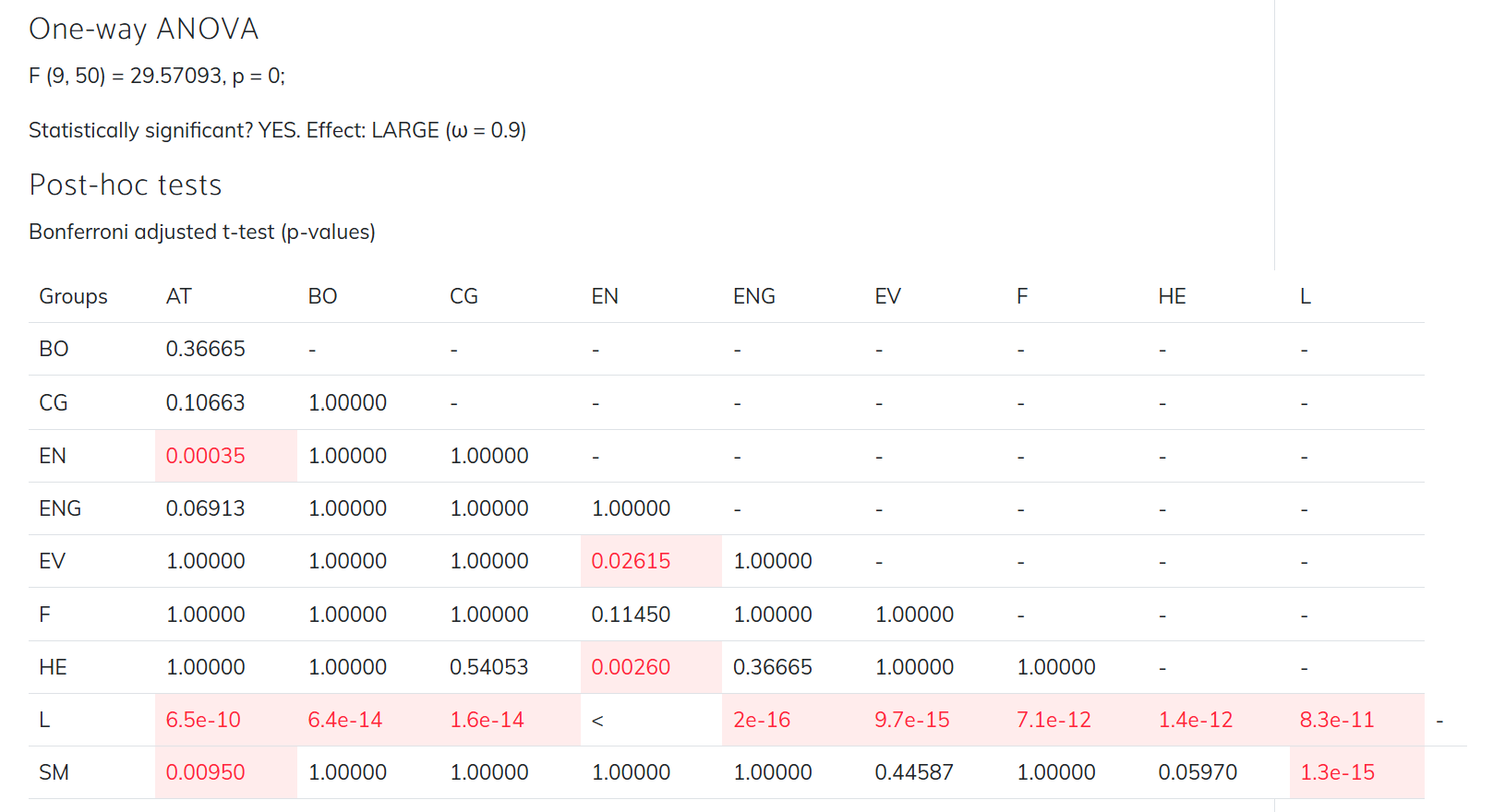
Example: In the provided results, a one-way ANOVA was conducted with 10 groups (dfbetween = 9, dfwithin = 50), yielding F(9, 50) = 29.57, p = 0. This indicates a highly significant result, meaning at least one group mean differs from the others. The effect size is large (ω = 0.9), suggesting a strong group effect.

Formula for F-statistic:

$F = \frac{\text{Mean Square Between Groups}}{\text{Mean Square Within Groups}}$

Post-hoc Tests

Bonferroni Adjusted t-tests

When a one-way ANOVA indicates significant differences among group means, post-hoc tests are used to identify which specific groups differ. The Bonferroni adjustment controls the family-wise error rate by dividing the significance level by the number of comparisons, making the test more conservative.

• Purpose: To determine which pairs of groups have statistically significant differences in their means.

• Interpretation: A p-value less than the adjusted significance level (commonly 0.05) indicates a significant difference between the corresponding groups.

Example: The table below shows Bonferroni-adjusted p-values for all pairwise group comparisons. Values highlighted (e.g., p < 0.05) indicate significant differences.

Groups	AT	BO	CG	EN	ENG	EV	F	HE	L	SM
BO	0.36665	-	-	-	-	-	-	-	-	-
CG	0.10663	1.00000	-	-	-	-	-	-	-	-
EN	0.00035	1.00000	1.00000	-	-	-	-	-	-	-
ENG	0.06913	1.00000	1.00000	1.00000	-	-	-	-	-	-
EV	1.00000	1.00000	1.00000	0.02615	1.00000	-	-	-	-	-
F	1.00000	1.00000	1.00000	0.11450	1.00000	1.00000	-	-	-	-
HE	1.00000	1.00000	0.54053	0.00260	0.36665	1.00000	1.00000	-	-	-
L	6.5e-10	6.4e-14	1.6e-14	<	2e-16	9.7e-15	7.1e-12	1.4e-12	-	-
SM	0.00950	1.00000	1.00000	1.00000	1.00000	0.44587	1.00000	0.05970	1.3e-15	-

How to Read the Table: Each cell shows the Bonferroni-adjusted p-value for the comparison between the row and column group. Values less than 0.05 (highlighted) indicate significant differences between those groups.

Summary

• The one-way ANOVA found a statistically significant difference among the group means (p = 0).

• Post-hoc Bonferroni tests identified which specific group pairs differ significantly.

• Effect size (ω = 0.9) indicates a large effect, meaning group membership explains a substantial portion of the variance.

Additional info: The Bonferroni method is one of several post-hoc procedures (others include Tukey's HSD and Scheffé's test), but it is particularly conservative and widely used when controlling for Type I error is a priority.