Chapter 2: Organizing and Summarizing Data in Introductory Statistics

Organizing and Summarizing Data

Introduction to Data Organization

When data is collected from surveys or experiments, it must be organized into a manageable form for analysis. Unorganized data is referred to as raw data. Organizing data allows statisticians to summarize, visualize, and interpret information efficiently.

Describing Data with Tables and Graphs

Organizing Qualitative Data

Qualitative data can be organized using frequency distributions, which list each category and the number of occurrences for each category.

• Frequency Distribution: A table that displays the frequency (count) of each category.

• Relative Frequency: The proportion or percentage of observations within a category, calculated as: $\text{Relative Frequency} = \frac{\text{Frequency of the category}}{\text{Total number of observations}}$

• Relative Frequency Distribution: A table that lists each category with its relative frequency.

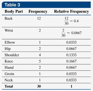
Example: A physical therapist records the body part requiring rehabilitation for 30 patients. The data is summarized in the following tables:

Body Part	Frequency	Relative Frequency
Back	12	0.4
Wrist	2	0.0667
Elbow	1	0.0333
Hip	2	0.0667
Shoulder	4	0.1333
Knee	5	0.1667
Hand	2	0.0667
Groin	1	0.0333
Neck	1	0.0333

Bar Graphs and Pareto Charts

Bar Graph: A graphical representation where each category is represented by a rectangle. The height of the rectangle corresponds to the frequency or relative frequency.

• Categories are labeled on one axis, and frequencies on the other.

• Bars are of equal width and do not touch.

Pareto Chart: A bar graph where bars are arranged in decreasing order of frequency or relative frequency, highlighting the most significant categories.

Side-by-Side and Horizontal Bar Graphs

Side-by-side bar graphs are used to compare two or more data sets, often using relative frequencies for fair comparison. Horizontal bar graphs are preferable when category names are lengthy.

Pie Charts

A pie chart is a circular graph divided into sectors, where each sector represents a category. The area of each sector is proportional to the frequency or relative frequency of the category.

• Degree measure for each sector: $\text{Degree} = \text{Relative Frequency} \times 360^\circ$

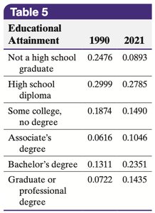
Educational Attainment	Frequency	Relative Frequency	Degree Measure
Not a high school graduate	20,054	0.0893	32
High school diploma	62,547	0.2785	100
Some college, no degree	33,455	0.1490	54
Associate's degree	23,487	0.1046	38
Bachelor's degree	52,805	0.2351	85
Graduate or professional degree	32,232	0.1435	52

Organizing Quantitative Data

Discrete vs. Continuous Data

Quantitative data can be discrete (countable values) or continuous (measurable values within an interval). For discrete data with few values, each value can be a category. For many values or continuous data, group data into classes (intervals).

Frequency and Relative Frequency Distributions for Quantitative Data

Frequency and relative frequency distributions can be constructed for discrete or continuous data. For continuous data, classes are defined by intervals with equal width.

• Class Limits: The smallest and largest values in a class.

• Class Width: The difference between consecutive lower class limits.

Example: Number of arrivals at Wendy's in 40 intervals:

Number of Customers	Frequency	Relative Frequency
1	1	0.025
2	6	0.15
3	1	0.025
4	4	0.1
5	7	0.175
6	11	0.275
7	5	0.125
8	2	0.05
9	2	0.05
10	0	0.0
11	1	0.025

Histograms

A histogram is a graphical representation of the frequency or relative frequency of quantitative data. Rectangles are drawn for each class, with heights representing frequencies and widths equal for all classes. Unlike bar graphs, histogram bars touch each other.

Dot Plots

A dot plot displays each observation as a dot above its value on a number line. It is useful for small data sets and shows the distribution's shape.

Shapes of Distributions

Distributions can be classified by their shape:

• Uniform: Frequencies are evenly spread.

• Bell-shaped: Highest frequency in the middle, tails off symmetrically.

• Skewed Right: Tail on the right is longer.

• Skewed Left: Tail on the left is longer.

Qualitative data is not described as skewed or bell-shaped.

Stem-and-Leaf Plots

A stem-and-leaf plot represents quantitative data by splitting each value into a "stem" (all but the rightmost digit) and a "leaf" (the rightmost digit). This plot preserves the original data and shows distribution shape.

• Split Stem: Used when data is bunched, by dividing stems into smaller intervals.

Frequency Polygons

A frequency polygon uses points connected by line segments to represent class frequencies. Points are plotted at class midpoints, and the graph is closed by connecting to the horizontal axis at each end.

• Class Midpoint: $\text{Midpoint} = \frac{\text{Lower class limit} + \text{Upper class limit}}{2}$

Cumulative Frequency and Ogives

Cumulative frequency distributions show the total number of observations less than or equal to a category or class. Cumulative relative frequency shows the proportion or percentage of observations less than or equal to a category or class.

An ogive is a graph of cumulative frequency or cumulative relative frequency, plotted at the upper class limits and connected by line segments.

Time-Series Plots

Time-series data are values measured at different points in time. A time-series plot displays time on the horizontal axis and the variable's value on the vertical axis, with points connected by line segments to show trends over time.

Misrepresentation of Data in Graphs

Common Misleading Practices

• Using bars with unequal widths or three-dimensional effects that distort perception.

• Manipulating the vertical scale (e.g., not starting at zero) to exaggerate differences.

• Combining categories inappropriately or using relative frequencies incorrectly.

• Failing to label axes or provide units and data sources.

Guidelines for Good Graphics:

• Title and label axes clearly, including units and sources.

• Avoid distortion and minimize white space.

• Indicate truncated scales clearly.

• Avoid clutter and unnecessary design elements.

• Prefer two-dimensional graphs over three-dimensional ones.

Example: A bar graph that does not start at zero may exaggerate differences between groups. Three-dimensional pie charts can mislead by making some categories appear larger than they are.

Additional info: These principles are foundational for accurate and ethical data presentation in statistics, ensuring that visualizations communicate the true story of the data without misleading the audience.