Paired Samples and Blocks: Inference for Dependent Samples

Paired Samples and Blocks

Introduction to Paired Data

Paired data arise when observations are collected in pairs, or when observations in one group are naturally related to those in another group. This structure is common in experiments where subjects are measured before and after a treatment, or when two measurements are taken on the same subject under different conditions. Recognizing paired data is crucial for selecting the correct statistical analysis.

• Paired Data: Observations are linked or matched in a meaningful way.

• Blocking: In experiments, pairing is a form of blocking to control for variability.

• Matching: In observational studies, pairing is often called matching.

Examples of Paired Data

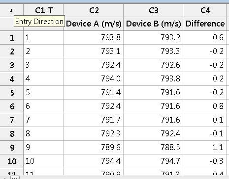
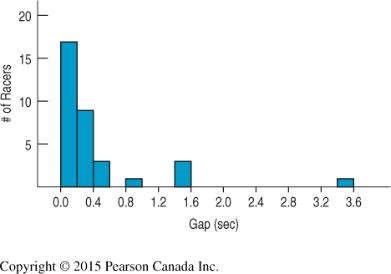
• Example 1: Measuring the muzzle velocity of the same round using two different devices. The data are paired because each round is measured by both devices.

• Example 2: Measuring reaction times of the same participant to two different stimuli (e.g., blue and red screens). The data are paired because each participant provides both measurements.

• Example 3: Measuring water clarity at the same location and dates, then repeating the measurements five years later. The data are paired because each measurement is matched by location and date.

Identifying Paired Data

To determine if data are paired, consider how the data were collected and what the observations represent. There is no formal test for pairing; it is a matter of study design and context. Once paired data are identified, analysis focuses on the differences within each pair, treating these differences as a single sample.

• Key Point: The analysis is based on the differences, not the original values.

Statistical Inference for Paired Data

The Paired t-Test

The paired t-test is used to test hypotheses about the mean difference between paired observations. Mechanically, it is a one-sample t-test applied to the differences.

• Sample Size (n): The number of pairs.

• Test Statistic: Calculated using the mean and standard deviation of the differences.

Test Statistic Formula:

$t = \frac{\bar{d} - \Delta_0}{s_d / \sqrt{n}}$

• $\bar{d}$ = mean of the differences

• $s_d$ = standard deviation of the differences

• $n$ = number of pairs

• $\Delta_0$ = hypothesized mean difference (often 0)

Assumptions and Conditions

• Paired Data Assumption: Data must be paired.

• Independence Assumption: Differences must be independent of each other.

• Randomization Condition: Data should be randomly sampled or assigned.

• 10% Condition: Sample should be less than 10% of the population (if sampling without replacement).

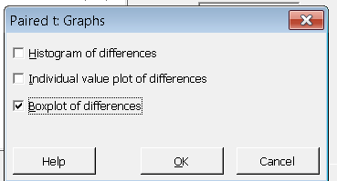
• Normal Population Assumption: The population of differences should be approximately normal. Check with a boxplot or normal probability plot.

Types of Hypothesis Tests

• Two-tailed Test: $H_0: \mu_d = \Delta_0$ vs $H_a: \mu_d \neq \Delta_0$

• Upper-tailed Test: $H_0: \mu_d = \Delta_0$ vs $H_a: \mu_d > \Delta_0$

• Lower-tailed Test: $H_0: \mu_d = \Delta_0$ vs $H_a: \mu_d < \Delta_0$

Confidence Interval for the Mean Difference

A confidence interval provides a plausible range for the true mean difference between paired observations.

Confidence Interval Formula:

$\bar{d} \pm t_{\alpha/2, n-1} \cdot \frac{s_d}{\sqrt{n}}$

• $t_{\alpha/2, n-1}$ = critical value from the t-distribution with $n-1$ degrees of freedom

Worked Examples

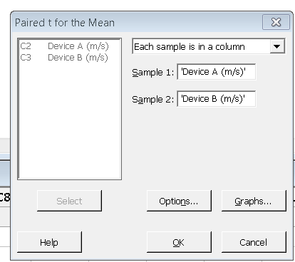
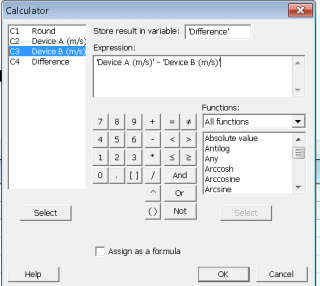
Example: Muzzle Velocity

Testing whether there is a difference in velocity measurements between Device A and Device B using paired data.

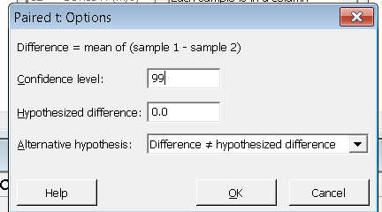
• Hypotheses: $H_0: \mu_d = 0$, $H_a: \mu_d \neq 0$

• Summary Statistics:

  • Device A: Mean = 792.458, SD = 1.407

  • Device B: Mean = 792.342, SD = 1.603

  • Difference: Mean = 0.117, SD = 0.475, n = 12

• Test Statistic: $t = 0.85$

• p-value: 0.413 (fail to reject $H_0$ at $\alpha = 0.01$)

• 99% Confidence Interval: (-0.309, 0.542) (contains 0, so no significant difference)

Example: Secchi Disk (Water Clarity)

Testing whether water clarity improved after 5 years using paired measurements at the same locations and dates.

• Hypotheses: $H_0: \mu_{diff} = 0$, $H_a: \mu_{diff} > 0$

• Summary Statistics:

  • Initial Mean = 54.38 in, SD = 12.69

  • 5 Years Later Mean = 59.50 in, SD = 8.73

  • Difference Mean = 5.13 in, SD = 6.08, n = 8

• Test Statistic: $t = 2.38$

• p-value: 0.024 (reject $H_0$ at $\alpha = 0.05$)

• Conclusion: Water clarity has significantly improved.

Effect Size and Sample Size

Confidence intervals help assess the size of the effect. The required sample size for a desired margin of error (ME) can be calculated as:

$n = \left( \frac{z^* s}{ME} \right)^2$

Additional info: Use $z^*$ instead of $t^*$ when degrees of freedom are unknown.

Blocking

Blocking is a design strategy where similar experimental units are grouped (blocked) together to reduce variability. Pairing is a special case of blocking, such as matching husbands and wives to compare their ages. Side-by-side boxplots of unpaired groups do not provide information about paired differences.

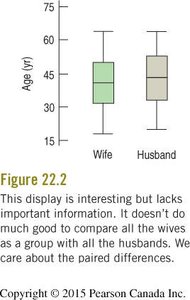
• Key Point: Pairing removes extra variation and focuses on the differences within pairs.

• Degrees of Freedom: Paired designs have fewer degrees of freedom than two-sample designs, but the reduction in variability often leads to more powerful tests.

Common Mistakes and Best Practices

• Do not use a two-sample t-test for paired data.

• Do not use paired methods for unpaired samples.

• Check for outliers in the distribution of differences.

• Do not compare means of paired groups with side-by-side boxplots; focus on the differences.

Summary of Key Concepts

• Recognize when data are paired or matched.

• Construct confidence intervals for the mean difference in paired data.

• Perform hypothesis tests about the mean difference, usually with a null hypothesis of zero difference.