Probability and Probability Distributions: Core Concepts for Introductory Statistics

Understanding Probability

Introduction to Probability

Probability is a fundamental concept in statistics that quantifies the likelihood of events occurring in random experiments. It is used to model uncertainty and make informed predictions about outcomes.

• Probability is a numerical value between 0 and 1 that describes the chance an event will occur.

• A random process or experiment produces outcomes called events.

• The sample space is the collection of all possible events.

• The probabilities of all events in the sample space must sum to 1.

• A probability of 1 means the event will certainly happen; a probability of 0 means it will not happen.

The Law of Large Numbers

The Law of Large Numbers states that as the number of observations increases, the proportion of times a particular outcome occurs approaches the true probability of that outcome.

• This principle underlies the reliability of probability estimates from repeated experiments.

The Language of Probability

Events, Sample Spaces, and Complements

Understanding the structure of events and their relationships is crucial for calculating probabilities.

• Event: A specific outcome or set of outcomes from a random process.

• Sample Space (S): The set of all possible outcomes.

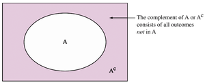
• Complement of an Event (Ac): All outcomes not in event A.

• Notation: If A is an event, then P(A) is the probability of A, and P(Ac) = 1 - P(A).

Mutually Exclusive (Disjoint) Events

Two events are mutually exclusive if they cannot occur at the same time. For such events, the probability of their intersection is zero.

• Example: Event 1 – person is a biological male; Event 2 – person is pregnant. These events are mutually exclusive.

• P(Event 1 ∩ Event 2) = 0

Sample Space Example: Deck of Cards

When drawing a card from a standard deck of 52 cards, the sample space includes all possible cards. Events can be defined based on characteristics such as color, suit, or face value.

• B = The card is black

• S = The card is a spade

• R = The card is red

• F = The card is a face card

Intersection and Union of Events

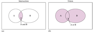
The intersection of two events (A ∩ B) is the set of outcomes shared by both events. The union of two events (A ∪ B) is the set of outcomes in either event or both.

• Intersection (A ∩ B): Outcomes in both A and B.

• Union (A ∪ B): Outcomes in A, B, or both.

• General Addition Rule: $P(A \cup B) = P(A) + P(B) - P(A \cap B)$

Calculating Probabilities with Unions and Intersections

To find the probability of the union of two events, use the general addition rule. If events are mutually exclusive, their intersection is zero.

• Example: If P(R) = 2/6, P(B) = 3/6, and P(R ∩ B) = 0, then $P(R \cup B) = 2/6 + 3/6 - 0 = 5/6$

• For non-mutually exclusive events, subtract the intersection to avoid double-counting.

Conditional Probability and Independence

Conditional Probability

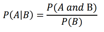
Conditional probability is the probability of one event occurring given that another event has occurred. It is denoted as P(A|B).

• Formula: $P(A|B) = \frac{P(A \cap B)}{P(B)}$

• "Given that" is represented by the vertical bar |.

Independence of Events

Two events are independent if the occurrence of one does not affect the probability of the other. For independent events, the probability of their intersection is the product of their probabilities.

• Formula: $P(A \cap B) = P(A) \times P(B)$

• Example: Coin tosses are independent events.

• If $P(A|B) = P(A)$, then A and B are independent.

Probability Distributions and Random Variables

Random Variables

A random variable is a numerical measurement of the outcome of a random phenomenon. The probability distribution of a random variable lists the probabilities associated with each possible value.

• Discrete random variables take on countable values.

• The sum of all probabilities in a probability distribution must be 1.

Expected Value (Mean) of a Random Variable

The expected value (E(X) or µ) of a random variable is the long-run average value of repetitions of the experiment it represents.

• Formula: $E(X) = \sum [x \cdot p(x)]$

• Example: If X is the number of heads in three coin flips, calculate E(X) using the probabilities for each possible value of X.

Applications of Expected Value

Expected value is used in real-world contexts such as insurance and games of chance to determine average outcomes over time.

• Example: Calculating the expected profit for an insurance company or expected winnings in a game.

The Normal Probability Distribution

Properties of the Normal Distribution

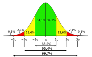
The normal distribution is a continuous probability distribution that is symmetric and bell-shaped. It is defined by its mean (µ) and standard deviation (σ).

• Mean = Median = Mode

• The area under the curve is always 1.

• Notation: $X \sim N(\mu, \sigma^2)$

The Empirical Rule (68-95-99.7 Rule)

The empirical rule describes the proportion of data within certain standard deviations of the mean in a normal distribution:

• About 68% of values fall within 1 standard deviation of the mean.

• About 95% within 2 standard deviations.

• About 99.7% within 3 standard deviations.

Calculating Probabilities with the Normal Distribution

Probabilities for normal distributions are found using the mean and standard deviation, often with statistical software or tables.

• To find the probability that X is between two values, calculate the area under the curve between those values.

• Percentiles and cutoff values can be determined using the cumulative distribution function (CDF).

Applications of the Normal Distribution

The normal distribution is widely used to model real-world phenomena such as heights, test scores, and commute times. It allows for the calculation of probabilities and percentiles for continuous data.

• Example: Calculating the probability of a commute time falling within a certain range, or determining the cutoff for the top 3% of values.

Summary Table: Key Probability Concepts

Concept	Definition	Formula
Complement	All outcomes not in event A	$P(A^c) = 1 - P(A)$
Intersection	Outcomes in both A and B	$P(A \cap B)$
Union	Outcomes in A, B, or both	$P(A \cup B) = P(A) + P(B) - P(A \cap B)$
Conditional Probability	Probability of A given B	$P(A|B) = \frac{P(A \cap B)}{P(B)}$
Independence	Events do not affect each other	$P(A \cap B) = P(A) \times P(B)$
Expected Value	Long-run average value	$E(X) = \sum [x \cdot p(x)]$
Normal Distribution	Symmetric, bell-shaped curve	$X \sim N(\mu, \sigma^2)$