Probability Concepts – Study Notes

Probability Concepts

Section 4.1: Probability Basics

Probability is a measure of how likely an event is to occur, expressed as a number between 0 and 1. In experiments with equally likely outcomes, probability quantifies the chance of a specific event occurring.

• Probability for Equally Likely Outcomes: If an experiment has N equally likely outcomes and an event can occur in f ways, the probability of the event is given by:

$P(E) = \frac{f}{N}$

• Basic Properties of Probabilities:

  • The probability of any event is between 0 and 1, inclusive.

  • The probability of an impossible event is 0.

  • The probability of a certain event is 1.

Example: Rolling a pair of dice has 36 possible outcomes. The probability of rolling a sum of 7 is the number of ways to get 7 divided by 36.

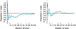
Example: Simulating coin tosses demonstrates that as the number of tosses increases, the proportion of heads approaches 0.5.

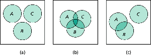
Section 4.2: Events

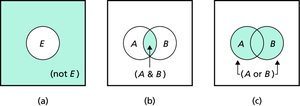
Events are subsets of the sample space, which is the set of all possible outcomes of an experiment.

• Sample Space (S): The collection of all possible outcomes.

• Event (E): Any subset of the sample space. An event occurs if the outcome is in E.

• Relationships Among Events:

  • Not E: The event that E does not occur (complement).

  • A & B: Both A and B occur (intersection).

  • A or B: Either A or B or both occur (union).

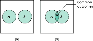
• Mutually Exclusive Events: Two or more events are mutually exclusive if they have no outcomes in common.

Section 4.3: Some Rules of Probability

Probability rules help calculate the likelihood of combined events.

• Probability Notation: $P(E)$ denotes the probability that event E occurs.

• Special Addition Rule: For mutually exclusive events A and B:

$P(A \text{ or } B) = P(A) + P(B)$

• For mutually exclusive events $A_1, A_2, ..., A_k$:

$P(A_1 \text{ or } A_2 \text{ or } ... \text{ or } A_k) = P(A_1) + P(A_2) + ... + P(A_k)$

• Complementation Rule: For any event E:

$P(\text{not } E) = 1 - P(E)$

• General Addition Rule: For any events A and B:

$P(A \text{ or } B) = P(A) + P(B) - P(A \text{ and } B)$

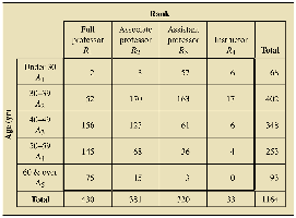
Section 4.4: Contingency Tables; Joint and Marginal Probabilities

Contingency tables organize data to show the frequency or probability of combinations of two or more categorical variables. Joint probabilities refer to the probability of two events occurring together, while marginal probabilities refer to the probability of a single event irrespective of the other.

Age/Rank	Full Professor	Associate Professor	Assistant Professor	Instructor	Total
Under 40	?	?	?	?	?
40–49	?	?	?	?	?
50–59	?	?	?	?	?
60 & over	?	?	?	?	?
Total	?	?	?	?	?

Age/Rank	Full Professor	Associate Professor	Assistant Professor	Instructor	P(Ai)
Under 40	0.002	0.009	0.029	0.005	0.045
40–49	0.045	0.146	0.149	0.013	0.343
50–59	0.135	0.107	0.031	0.005	0.278
60 & over	0.066	0.029	0.003	0.000	0.098
P(Rj)	0.249	0.291	0.212	0.023	1.000

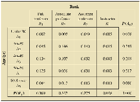
Section 4.5: Conditional Probability

Conditional probability is the probability that event B occurs given that event A has occurred. It is denoted as $P(B|A)$ and calculated using:

$P(B|A) = \frac{P(A \text{ and } B)}{P(A)}$

• Example: The probability that a faculty member is an associate professor given they are aged 40–49 can be found using the joint and marginal probabilities from the contingency table.

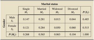
Gender	Single	Married	Widowed	Divorced	P(Si)
Male	0.147	0.281	0.013	0.044	0.485
Female	0.121	0.284	0.050	0.060	0.515
P(Mj)	0.268	0.565	0.063	0.104	1.000

Section 4.6: The Multiplication Rule; Independence

The multiplication rule is used to find the probability that two events both occur. If A and B are independent, the probability that both occur is the product of their probabilities.

• General Multiplication Rule: $P(A \text{ and } B) = P(A) \times P(B|A)$

• Independent Events: Events A and B are independent if $P(B|A) = P(B)$.

• Special Multiplication Rule (for Independent Events): $P(A \text{ and } B) = P(A) \times P(B)$

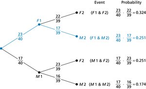
Example: Tree diagrams can be used to visualize and calculate probabilities for sequences of events.

Section 4.7: Bayes’s Rule

Bayes’s Rule allows us to update probabilities based on new information. It is especially useful when dealing with conditional probabilities and partitioned sample spaces.

• Rule of Total Probability: If $A_1, A_2, ..., A_k$ are mutually exclusive and exhaustive events, then for any event B:

$P(B) = P(B|A_1)P(A_1) + P(B|A_2)P(A_2) + ... + P(B|A_k)P(A_k)$

• Bayes’s Rule: For mutually exclusive and exhaustive events $A_1, ..., A_k$:

$P(A_i|B) = \frac{P(B|A_i)P(A_i)}{P(B|A_1)P(A_1) + ... + P(B|A_k)P(A_k)}$

Section 4.8: Counting Rules

Counting rules are essential for determining the number of possible outcomes in probability problems.

• Basic Counting Rule (BCR): If r actions are performed in order, with $n_1$ possibilities for the first, $n_2$ for the second, ..., $n_r$ for the r-th, then the total number of possibilities is $n_1 \times n_2 \times ... \times n_r$.

• Factorials: $k! = k \times (k-1) \times ... \times 2 \times 1$; by definition, $0! = 1$.

• Permutations: The number of ways to arrange r objects from m is:

$P(m, r) = \frac{m!}{(m-r)!}$

• Special Permutations: The number of ways to arrange m objects is $m!$.

• Combinations: The number of ways to choose r objects from m (order does not matter):

$C(m, r) = \frac{m!}{r!(m-r)!}$

• Number of Possible Samples: The number of samples of size n from a population of size N is $C(N, n)$.

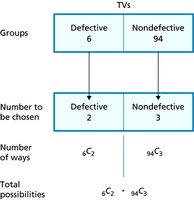
Example: Calculating the number of ways to select exactly 2 defective TVs from 5 selected TVs, given 6 defective and 94 nondefective TVs in total.