Probability, Discrete and Binomial Distributions, and the Normal Curve

Probability and Probability Rules

Random Processes and the Law of Large Numbers

Probability theory is the foundation of statistical inference. A random process is an experiment or procedure whose outcome cannot be predicted with certainty. The Law of Large Numbers states that as the number of trials in a random process increases, the experimental probability of an event approaches its theoretical probability.

• Experimental Probability: Probability based on observed outcomes of an experiment.

• Theoretical Probability: Probability calculated based on possible outcomes in the sample space.

• Sample Space: The set of all possible outcomes of a random process.

• Probability: A measure between 0 and 1 that quantifies the likelihood of an event.

• Complement: The set of outcomes in the sample space that are not in the event.

Rules for Probability:

• Probability of any event: $0 \leq P(A) \leq 1$

• Sum of probabilities of all possible outcomes: $\sum P(x) = 1$

Example: If a pair of fair dice is rolled, the sample space consists of 36 outcomes. The probability of rolling a sum of 7 is $P(7) = \frac{6}{36} = 0.167$.

Probability Models

A probability model assigns probabilities to all possible outcomes of a random process. Probabilities must be non-negative and sum to 1.

x	0	1	2	3
P(x)	0.2	0.15	?	0.25

To find the missing probability, use $\sum P(x) = 1$.

Addition and Complement Rules

The Addition Rule is used to find the probability that at least one of two events occurs:

• $P(A \text{ or } B) = P(A) + P(B) - P(A \text{ and } B)$

The Complement Rule states:

• $P(A^c) = 1 - P(A)$

Mutually Exclusive (Disjoint) Events: Events that cannot occur at the same time, so $P(A \text{ and } B) = 0$.

Probability Table Example

Color	R	G	BL	BR	Y	O
P(c)	0.3	0.15	0	0.15	0.2	0.2

Verify the model by checking that all probabilities sum to 1.

Multiplication Rule and Independence

Independent and Dependent Events

Events are independent if the occurrence of one does not affect the probability of the other. Otherwise, they are dependent.

• Multiplication Rule: $P(A \text{ and } B) = P(A) \times P(B|A)$

• Conditional Probability: $P(B|A)$ is the probability of B given A has occurred.

Example: The probability of rolling three ones in a row on a fair die is $\left(\frac{1}{6}\right)^3 = \frac{1}{216}$.

Discrete Probability Distributions

Expected Value and Standard Deviation

A discrete probability distribution lists each possible value of a random variable and its probability. The expected value (mean) and standard deviation measure the center and spread of the distribution.

• Expected Value (Mean): $\mu = \sum x_i p_i$

• Standard Deviation: $\sigma = \sqrt{\sum (x_i - \mu)^2 p_i}$

Example: For a basketball player shooting free throws, let x be the number of shots made and p(x) the probability for each value. Calculate mean and standard deviation using the formulas above.

Binomial Distribution

Identifying Binomial Scenarios

A binomial experiment consists of n independent trials, each with two possible outcomes (success or failure) and constant probability of success p.

• Binomial Probability Formula: $P(r) = \binom{n}{r} p^r (1-p)^{n-r}$

• Mean: $\mu = np$

• Standard Deviation: $\sigma = \sqrt{np(1-p)}$

Example: If a basketball player makes 80% of free throws and shoots 3 times, use the binomial formula to find the probability of making exactly 2 shots.

The Normal Curve and Empirical Rule

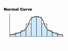
Introduction to the Normal Curve

The normal curve is a symmetric, bell-shaped curve that describes many natural phenomena. It is defined by its mean (center) and standard deviation (spread). The area under the curve represents probability and always equals 1.

• The center of the curve is the mean ($\mu$).

• The curve follows the Empirical Rule (68-95-99.7 Rule):

  • About 68% of data falls within 1 standard deviation of the mean.

  • About 95% within 2 standard deviations.

  • About 99.7% within 3 standard deviations.

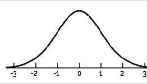
Z-Scores and Standard Normal Distribution

A z-score measures how many standard deviations a value is from the mean:

• $z = \frac{x - \mu}{\sigma}$

The standard normal distribution has mean 0 and standard deviation 1. Z-scores are used to find probabilities and percentiles for normal distributions.

Applications of the Normal Distribution

To find probabilities for normal distributions:

• Convert the value to a z-score.

• Use the standard normal table or technology to find the area (probability) under the curve.

Example: The length of a 4-year-old male's upper arm is approximately normal with mean 21.8 cm and standard deviation 2.0 cm. To find the probability that a randomly selected boy has an upper arm length less than 19.8 cm, calculate the z-score and use the normal table.

Percentiles and Inverse Normal Calculations

The percentile of a value is the percentage of data below that value. To find the value corresponding to a given percentile, use the inverse normal function:

• Find the z-score for the desired percentile.

• Calculate $x = \mu + z\sigma$.

Example: The height of 3-year-old girls is approximately normal with mean 38.7 in and standard deviation 3.2 in. To find the height at the 90th percentile, use the inverse normal calculation.

Summary Table: Key Probability Rules and Formulas

Rule	Formula	Description
Addition Rule	$P(A \text{ or } B) = P(A) + P(B) - P(A \text{ and } B)$	Probability of A or B occurring
Complement Rule	$P(A^c) = 1 - P(A)$	Probability of the complement of A
Multiplication Rule	$P(A \text{ and } B) = P(A) \times P(B|A)$	Probability of both A and B occurring
Expected Value	$\mu = \sum x_i p_i$	Mean of a discrete random variable
Standard Deviation	$\sigma = \sqrt{\sum (x_i - \mu)^2 p_i}$	Spread of a discrete random variable
Binomial Probability	$P(r) = \binom{n}{r} p^r (1-p)^{n-r}$	Probability of r successes in n trials
Z-Score	$z = \frac{x - \mu}{\sigma}$	Standardized value for normal distributions

Additional info: This guide covers probability rules, discrete and binomial distributions, and the normal curve, including calculation of probabilities, expected values, standard deviations, and applications of the normal distribution.