Probability Distributions and the Normal Distribution

Probability Distributions

Random Variables and Probability Distributions

A random variable is a variable whose value is a numerical outcome of a random phenomenon. The probability distribution of a random variable X describes the possible values X can take and the probabilities associated with those values.

• Discrete random variable: Can assume only a finite or countable number of values.

• Continuous random variable: Can assume any value within one or more intervals.

Examples of discrete random variables:

• Number of cheeseburgers sold at a restaurant today

• Number of home football games won by a team in a season

• Number of points missed on a quiz

• Number of cars washed at a car wash today

Probability Distribution of a Discrete Random Variable:

• Each possible value x has a probability p(x) such that 0 ≤ p(x) ≤ 1

• The sum of all probabilities for possible x values equals 1

Example (Benford's Law): The probability distribution for the first digit X in legitimate financial records is:

First digit (x)	1	2	3	4	5	6	7	8	9
Probability	0.301	0.176	0.125	0.097	0.079	0.067	0.058	0.051	0.046

To verify this is a legitimate probability distribution, check that all probabilities are between 0 and 1 and their sum is 1.

Mean (Expected Value) of a Discrete Probability Distribution:

The mean (expected value) is given by:

$\mu = \sum x p(x)$

This is a weighted average of the possible values, where each value is weighted by its probability.

Standard Deviation: The standard deviation $\sigma$ measures the variability from the mean.

Probability Distributions of Categorical Variables: For variables with two categories (e.g., success/failure), outcomes can be coded as 0 and 1. The mean of this distribution equals the probability of success.

• Example: Probability a customer buys a product is 0.20. The mean is $0 \times 0.80 + 1 \times 0.20 = 0.20$.

Continuous Random Variables and Density Curves

A continuous random variable can take any value in an interval. Its probability distribution is described by a density curve:

• The probability that the variable falls within an interval is the area under the curve above that interval.

• The total area under the curve is 1.

In practice, continuous variables are measured discretely due to rounding, but the density curve provides a good approximation.

Density Curve Properties:

• Always on or above the horizontal axis

• Total area under the curve is 1

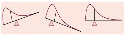
The median of a density curve is the point dividing the area in half. The mean is the balance point of the curve. For symmetric curves, mean and median coincide; for skewed curves, the mean is pulled toward the tail.

Uniform Distribution Example

Accidents occur uniformly along a 5-mile bike path. The density curve is flat, and the area under the curve between two points gives the proportion of accidents in that interval.

• Proportion in the first mile: Area from 0 to 1 mile

• Proportion alongside a stream: Area from 0.8 to 1.3 miles

• Proportion more than 1 mile from either end: Area outside the first and last mile

Normal Distributions

Properties of the Normal Distribution

The normal distribution is a symmetric, bell-shaped density curve determined by its mean $\mu$ and standard deviation $\sigma$. The mean is at the center, and the standard deviation controls the spread.

• Notation: $N(\mu, \sigma)$

• Inflection points (where curvature changes): $\mu - \sigma$ and $\mu + \sigma$

Importance of Normal Distributions:

• Good models for many real-world data sets

• Useful approximations for many chance outcomes

• Basis for many statistical inference procedures

The Empirical Rule (68-95-99.7 Rule)

For a normal distribution:

• About 68% of observations fall within 1 standard deviation of the mean

• About 95% fall within 2 standard deviations

• About 99.7% fall within 3 standard deviations

This rule also applies approximately to other mound-shaped, symmetric distributions.

z-Scores and the Standard Normal Distribution

The z-score for a value x from a distribution with mean $\mu$ and standard deviation $\sigma$ is:

$z = \frac{x - \mu}{\sigma}$

The z-score measures how many standard deviations x is from the mean. Positive z-scores are above the mean; negative are below.

The standard normal distribution is $N(0, 1)$, with mean 0 and standard deviation 1. Any normal variable can be standardized to a z-score, which then follows the standard normal distribution.

Finding Probabilities and Values

Probabilities for normal distributions correspond to areas under the curve. These can be found using technology or standard normal tables. To find a value x given a z-score:

$x = z \sigma + \mu$

To find probabilities for intervals, convert x-values to z-scores and use the standard normal distribution.

Normal Probability Plots

A normal probability plot graphs observed data against expected values from a normal distribution. If the data are normal, the plot is approximately a straight line. Deviations from linearity indicate departures from normality (e.g., skewness or multiple populations).

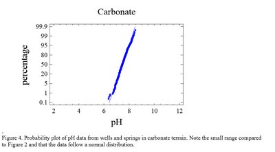
Example: The plot above shows pH data from wells in carbonate terrain. The data follow a normal distribution, as indicated by the straight line.

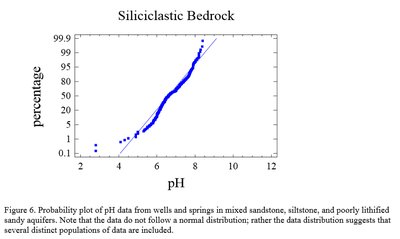
Example: The plot above shows pH data from wells in siliciclastic bedrock. The data do not follow a normal distribution; the plot is not linear, suggesting multiple populations or non-normality.

Additional info: Normal probability plots are a key diagnostic tool for assessing normality before applying statistical inference methods that assume normality.