Probability Distributions: Discrete, Binomial, and Normal Distributions

Probability Distributions

Random Variables and Probability Distributions

A random variable (RV) is a variable whose value is determined by chance. Probability distributions describe how probabilities are assigned to each possible value of a random variable.

• Discrete random variable: Has countable outcomes (e.g., number of heads in coin flips).

• Continuous random variable: Has infinitely many outcomes within an interval (e.g., height, weight).

• Probability distribution: A table or function pairing each outcome with its probability.

Requirements for a probability distribution:

1. There is a numerical random variable x, and each possible outcome has a probability.

2. The sum of all probabilities for the RV must be 1.

3. Each probability must be between 0 and 1.

Example: Coin Flips

For two flips of a coin, the random variable X = number of heads. The probability distribution is:

X (Number of Heads)	P(X)
0	0.25
1	0.5
2	0.25

Expected Value (Mean): The mean value of the outcomes, calculated as:

$E(X) = \sum x_i P(x_i)$

Standard Deviation: Measures the spread of the distribution:

$\sigma = \sqrt{\sum (x_i - \mu)^2 P(x_i)}$

Binomial Probability Distributions

A binomial probability distribution is a special case of discrete probability distributions, defined by parameters n (number of trials) and p (probability of success). It applies when:

• There is a fixed number of trials.

• Trials are independent.

• Each trial has two possible outcomes: success or failure.

• The probability of success remains constant for each trial.

The mean, variance, and standard deviation for a binomial distribution are:

$\mu = np$ $\sigma^2 = npq$ $\sigma = \sqrt{npq}$

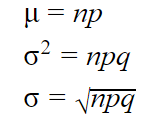
Where q = 1 - p (probability of failure).

Example: Archer Hitting Bull's-Eye

If an archer hits the bull's-eye 55% of the time and shoots 8 arrows, the probability of getting exactly 5 bull's-eyes is calculated using the binomial formula:

$P(X = k) = \binom{n}{k} p^k q^{n-k}$

For n = 8, p = 0.55, k = 5:

$P(X = 5) = \binom{8}{5} (0.55)^5 (0.45)^3$

Statistical software (e.g., StatCrunch) can be used for computation.

Example: NFL Overtime Games

In 460 games, 252 were won by the team winning the coin toss. This scenario satisfies binomial conditions:

• Fixed number of trials (n = 460).

• Two outcomes (win or lose).

• Independent trials.

• Constant probability (p = 0.5).

Mean and standard deviation:

$\mu = 460 \times 0.5 = 230$ $\sigma = \sqrt{460 \times 0.5 \times 0.5} = 10.724$

Continuous Probability Distributions

A continuous probability distribution describes the probabilities of outcomes for a continuous random variable. The most important example is the normal distribution, which is symmetric and bell-shaped.

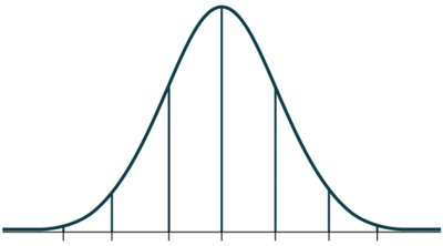
The normal distribution is defined by its mean (\( \mu \)) and standard deviation (\( \sigma \)).

A standard normal distribution is a normal distribution with \( \mu = 0 \) and \( \sigma = 1 \). Outcomes are transformed into z-scores:

$z = \frac{x - \mu}{\sigma}$

Example: Bone Density Test

Bone density scores are normally distributed and measured as z-scores. The probability that a randomly selected adult has a z-score less than 1.27 is found using the normal distribution table or software.

Probability between two z-scores (e.g., -2.50 and -1.00) indicates the likelihood of osteopenia.

Finding z-scores for Given Probabilities

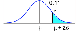
To find the z-score that separates the bottom 2.5% from the top 97.5%, use the standard normal table:

$P(z < -1.96) = 0.025$ $P(z > 1.96) = 0.025$

Example: Military Pilot Heights

Heights of men are normally distributed with \( \mu = 68.6 \) inches and \( \sigma = 2.8 \) inches. To find the percentage of men meeting height requirements (62 to 77 inches), calculate the probability that a value falls within this interval using z-scores.

To find the 15th percentile, solve for x:

$z = -1.036$ $x = \mu + z \sigma = 68.6 + (-1.036) \times 2.8 = 65.699$

Applications and Comparisons

• Discrete vs. Continuous: Discrete random variables have countable outcomes; continuous random variables have uncountable outcomes within intervals.

• Binomial vs. Normal: Binomial distributions can be approximated by normal distributions when n is large and p is not too close to 0 or 1.

Summary Table: Binomial vs. Normal Distribution

Distribution	Type	Parameters	Shape
Binomial	Discrete	n, p	Symmetric for p=0.5, skewed otherwise
Normal	Continuous	\( \mu \), \( \sigma \)	Symmetric, bell-shaped

Key Formulas:

• Binomial mean: $\mu = np$

• Binomial variance: $\sigma^2 = npq$

• Binomial standard deviation: $\sigma = \sqrt{npq}$

• Normal z-score: $z = \frac{x - \mu}{\sigma}$

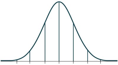
Example: Calculating the probability that a value falls above a certain z-score (e.g., right tail probability of 0.11) can be visualized as the shaded area under the normal curve.