Chapter 5 Study Guide

Probability Distributions

Introduction to Probability Distributions

A probability distribution describes how probabilities are assigned to each possible value of a random variable. It provides a model for understanding the likelihood of different outcomes in a chance process.

• Random Variable: A numerical outcome determined by chance, typically denoted by a capital letter (e.g., X).

• Discrete Random Variable: Has finite or countable possible values (e.g., number of seedlings germinating).

• Continuous Random Variable: Has infinitely many possible values on a continuum (e.g., plant height).

Example: If X = number of seedlings that germinate out of 3 planted seeds, possible values are 0, 1, 2, 3.

Requirements for a Valid Discrete Probability Distribution

• X is numerical: The values represent a numerical random variable.

• Sum of probabilities: $\sum P(x) = 1$ (allowing small rounding differences).

• Probability bounds: $0 \leq P(x) \leq 1$ for every individual probability.

Representing Probability Distributions

Probability distributions can be represented using tables, formulas, or graphs. For example:

x (seedlings germinating)	P(x)
0	0.10
1	0.25
2	0.40
3	0.25

Probability Histograms

A probability histogram visually displays a discrete probability distribution. The horizontal axis shows possible values of X, and the vertical axis shows P(x). Bar heights represent probabilities, not observed frequencies.

Describing a Probability Distribution: Mean, Variance, and Standard Deviation

The mean (expected value), variance, and standard deviation describe the center and spread of a probability distribution.

• Mean (Expected Value): $\mu = E(X) = \sum [x \cdot P(x)]$

• Variance: $\sigma^2 = \sum [(x - \mu)^2 \cdot P(x)]$ or $\sigma^2 = \sum [x^2 \cdot P(x)] - \mu^2$

• Standard Deviation: $\sigma = \sqrt{\sigma^2}$

Example: For the table above, $\mu = 1.80$, $\sigma^2 = 0.86$, $\sigma \approx 0.93$.

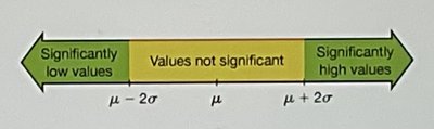
Identifying Unusual Outcomes: Range Rule of Thumb

The Range Rule of Thumb helps identify unusually low or high values in a probability distribution:

• Unusually low: $x \leq \mu - 2\sigma$

• Unusually high: $x \geq \mu + 2\sigma$

Values between these cutoffs are considered not significant. This is a heuristic, not a formal definition.

Probability-Based Unusual Outcomes: Alternatively, outcomes can be judged unusual if their probability is less than or equal to 0.05:

• Unusually high: $P(X \geq x) \leq 0.05$

• Unusually low: $P(X \leq x) \leq 0.05$

Binomial Probability Distributions

Binomial Model Requirements

A binomial probability distribution models the number of successes in a fixed number of independent trials, each with two outcome categories and a constant probability of success.

• Fixed number of trials (n)

• Independent trials

• Two outcome categories (success/failure)

• Constant probability of success (p)

Notation: n = number of trials, X = number of successes, x = particular value, p = probability of success, q = probability of failure ($q = 1 - p$).

Binomial Probability Formula

The probability of exactly x successes in n trials is:

$P(x) = \frac{n!}{(n-x)!x!} p^x q^{n-x}$

The combination component $\frac{n!}{(n-x)!x!}$ counts the number of ways to choose which x of the n trials are successes.

Mean and Standard Deviation of Binomial Distribution

• Mean: $\mu = np$

• Variance: $\sigma^2 = npq$

• Standard deviation: $\sigma = \sqrt{npq}$

Example: If n = 20 and p = 0.30, then $\mu = 6$, $\sigma \approx 2.05$.

Identifying Unusual Outcomes in Binomial Distributions

Use the range rule of thumb or cumulative probabilities:

• Unusually low: $x \leq \mu - 2\sigma$

• Unusually high: $x \geq \mu + 2\sigma$

• Probability-based: $P(X \geq x) \leq 0.05$ or $P(X \leq x) \leq 0.05$

Poisson Probability Distributions

Poisson Model Requirements

A Poisson probability distribution models the number of occurrences of an event within a specified interval (time, distance, area, or volume).

• Random occurrences

• Independent occurrences

• Uniformly distributed rate across the interval

Notation: X = number of occurrences, x = particular value, μ = mean number of occurrences per interval.

Poisson Probability Formula

The probability of exactly x occurrences in an interval is:

$P(x) = \frac{\mu^x e^{-\mu}}{x!}$

Where e is the mathematical constant (≈ 2.71828).

Mean and Standard Deviation of Poisson Distribution

• Mean: $\mu$

• Variance: $\sigma^2 = \mu$

• Standard deviation: $\sigma = \sqrt{\mu}$

Example: If μ = 9, then variance = 9, σ = 3.

Poisson Approximation to the Binomial

When n is large and p is small, a Poisson distribution can approximate a binomial distribution. For this course, use:

• $n \geq 100$

• $np \leq 10$

• Then $\mu = np$

Summary Table: Binomial vs. Poisson Models

Feature	Binomial	Poisson
What is counted?	Successes in fixed trials	Occurrences in fixed interval
Parameters	n, p	μ
Possible values	0, 1, ..., n	0, 1, 2, ... (no upper limit)
Mean	$np$	$\mu$
Variance	$npq$	$\mu$
Standard deviation	$\sqrt{npq}$	$\sqrt{\mu}$

Key Takeaways

• Probability distributions model the likelihood of outcomes for random variables.

• Discrete distributions include binomial and Poisson models, each with specific requirements and formulas.

• Mean, variance, and standard deviation describe the center and spread of distributions.

• Unusual outcomes can be identified using the range rule of thumb or probability-based criteria.