Probability Distributions of Discrete Random Variables

Probability Models of Data

Random Variables

A random variable is a function that assigns a unique numerical value to each outcome of a random experiment. Random variables allow us to quantify outcomes and analyze their distributions mathematically.

• Discrete random variables take on a countable number of possible values (e.g., number of heads in coin tosses).

• Continuous random variables can take on any value within a given range (e.g., time to commute).

Examples of random experiments and their sample spaces:

• Tossing a coin three times: S = {HHH, HHT, HTH, HTT, THH, THT, TTH, TTT} (finite, discrete)

• Tossing a coin until the first head appears: S = {H, TH, TTH, TTTH, ...} (countably infinite, discrete)

• Measuring commute time: S = all real numbers from 0 to ∞ (infinite, continuous)

Random variables are typically denoted by capital letters (e.g., X), and their possible values by lowercase letters with subscripts (e.g., xi).

Probability Distribution of a Random Variable

The probability distribution of a discrete random variable X is a table or function that lists each possible value xi and its probability P(X = xi).

For a valid probability distribution:

• 0 < P(X = xi) < 1 for all i

• Sum of all probabilities equals 1: $\sum_{i=1}^{k} P(X = x_i) = 1$

Example: Number of Heads in Three Coin Tosses

Let X be the number of heads observed in three tosses of a fair coin. The probability distribution is:

x	0	1	2	3
P(X = x)	0.125	0.375	0.375	0.125

The sum of probabilities is $0.125 + 0.375 + 0.375 + 0.125 = 1$.

Example: Rolling a Fair Die

Let X be the uppermost face when rolling a fair six-sided die. The probability distribution is:

x	1	2	3	4	5	6
P(X = x)	1/6	1/6	1/6	1/6	1/6	1/6

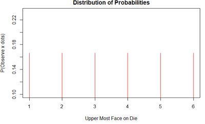
This distribution is uniform, meaning each outcome is equally likely.

Example: Lotto Max Lottery

Suppose you buy one Lotto Max ticket and count how many numbers match the 7 winning numbers. The probability distribution (partial) is:

x	0	1	2	3	4	5	6	7
P(X = x)	0.31406	0.42748	?	0.045606	0.00468	0.00021	0.000003	0.000000012

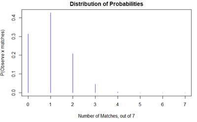
To find the missing probability for x = 2, use the fact that the probabilities must sum to 1:

$P(X = 2) = 1 - (0.31406 + 0.42748 + 0.045606 + 0.00468 + 0.00021 + 0.000003 + 0.000000012)$

Expected Value (Mean) of a Discrete Random Variable

The expected value (mean) of a discrete random variable X is the long-run average value of X over many repetitions of the experiment. It is calculated as:

$E[X] = \sum_{i=1}^{k} x_i P(X = x_i)$

Example: For the coin toss example above, the expected number of heads is:

$E[X] = 0 \times 0.125 + 1 \times 0.375 + 2 \times 0.375 + 3 \times 0.125 = 1.5$

Application: Lottery Ticket Expected Value

Suppose you buy a lottery ticket with the following payout structure:

• Match 0 numbers: win $0 (P = 0.6697)$

• Match 1 number: win $2 (P = 0.3013)$

• Match 2 numbers: win $10 (P = 0.0287)$

• Match 3 numbers: win $1000 (P = ?)$

To find the missing probability for matching all three numbers:

$P(X = 3) = 1 - (0.6697 + 0.3013 + 0.0287) = 0.0003$

The expected winnings are:

$E[X] = 0 \times 0.6697 + 2 \times 0.3013 + 10 \times 0.0287 + 1000 \times 0.0003$

Subtract the ticket cost to determine if the game is favorable.

Summary Table: Properties of Probability Distributions

Property	Description
Non-negativity	All probabilities are between 0 and 1
Normalization	Sum of all probabilities equals 1
Expected Value	Weighted average of possible values

Additional info: The notes above expand on the basic definitions and calculations for discrete probability distributions, including expected value and applications to games of chance. The images included directly illustrate the probability distributions for the die roll and Lotto Max examples, reinforcing the tabular data and supporting the explanation of probability models.