Probability Distributions, The Normal and Binomial Models, and Statistical Inference

Probability Distributions

Introduction to Probability Distributions

Probability distributions are mathematical models that describe the likelihood of different outcomes in a random experiment. They are fundamental in statistics for modeling and predicting random events.

• Random Variable: A variable whose value is determined by the outcome of a random experiment.

• Probability Distribution: Describes how probabilities are assigned to the possible values of a random variable.

• All probabilities in a distribution must sum to 1.

Types of Probability Distributions

• Discrete Probability Distributions: Model outcomes that take countable values (e.g., number of colonies, number of mutations).

• Continuous Probability Distributions: Model outcomes that can take any value within a range (e.g., temperature, biomass weight, cell diameter).

Examples of Discrete and Continuous Variables

• Discrete: Number of patients in a clinical trial, count of colonies on an agar plate.

• Continuous: Temperature of a fermenter, pH of culture medium.

Representing Probability Distributions

• Discrete random variables are often represented by tables, graphs, or formulas.

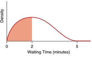
• Continuous random variables are represented by probability density functions (PDFs), where probabilities correspond to areas under the curve.

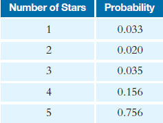
Example Table: Discrete Probability Distribution

Number of Stars	Probability
1	0.033
2	0.020
3	0.035
4	0.156
5	0.756

Finding Probabilities as Area

For continuous distributions, the probability of an event occurring within a range is the area under the curve between those values.

The Normal Distribution

Properties of the Normal Distribution

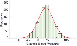
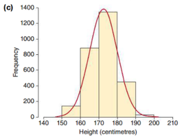
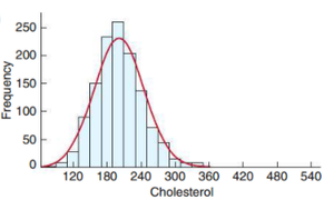
The normal distribution is a continuous probability distribution that is symmetric and unimodal. It is widely used to model natural phenomena and measurement errors.

• Characterized by its mean (μ) and standard deviation (σ).

• Notation: $N(\mu, \sigma)$

• The total area under the curve is 1.

Visualizing the Normal Distribution

Standard Normal Distribution and Z-scores

The standard normal distribution is a special case with mean 0 and standard deviation 1, denoted as $N(0,1)$. Z-scores standardize values for comparison.

• Z-score formula: $z = \frac{x - \mu}{\sigma}$

• Z-scores indicate how many standard deviations a value is from the mean.

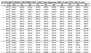
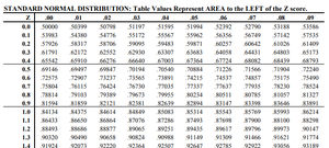
Using the Standard Normal Table

Probabilities for the standard normal distribution are found using a table that gives the area to the left of a given z-score.

Empirical Rule (68-95-99.7 Rule)

• About 68% of values fall within 1 standard deviation of the mean.

• About 95% within 2 standard deviations.

• About 99.7% within 3 standard deviations.

Example: Calculating Normal Probabilities

• Convert the value to a z-score.

• Look up the area in the standard normal table.

• For example, the probability that a newborn grizzly bear cub weighs less than 625 grams (given $N(650, 20)$) is 0.1056.

The Binomial Distribution

Properties of the Binomial Distribution

The binomial distribution models the number of successes in a fixed number of independent trials, each with the same probability of success.

• Each trial has two possible outcomes: success or failure.

• Notation: $b(n, p, x)$ is the probability of x successes in n trials with probability p of success.

• Mean: $\mu = np$

• Standard deviation: $\sigma = \sqrt{np(1-p)}$

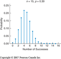
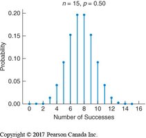
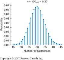
Shape of the Binomial Distribution

• Symmetric if $p = 0.5$ or if n is large, even if p is not 0.5.

• Skewed if p is far from 0.5 and n is small.

Example: Binomial Probability Calculation

Suppose 60% of bacterial cells take up a plasmid gene. In a sample of 15 colonies, the probability that exactly 8 express the gene is $b(15, 0.60, 8)$.

Statistical Inference

Population, Sample, Parameter, and Statistic

• Population: The entire group of interest.

• Sample: A subset of the population used to draw conclusions.

• Parameter: A numerical summary of the population (e.g., population mean μ).

• Statistic: A numerical summary of the sample (e.g., sample mean x̄).

Sampling Error and Bias

• Sampling Error: The natural variability in statistics from sample to sample.

• Bias: Systematic error that leads to inaccurate estimates (e.g., measurement bias, sampling bias).

Accuracy and Precision

• Accuracy: The method measures what it is intended to measure.

• Precision: The method yields consistent results when repeated.

Sampling Distributions and the Central Limit Theorem (CLT)

Sampling Distribution of a Statistic

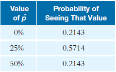
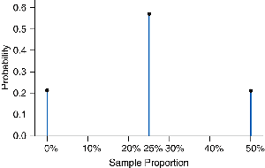
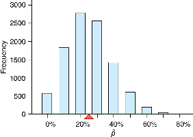
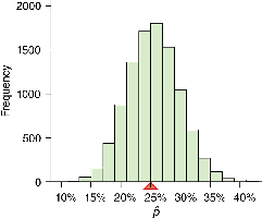
The sampling distribution describes the distribution of a statistic (e.g., sample mean or proportion) over many samples from the same population.

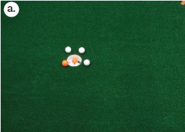
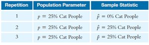
Simulation Example: Cat People

Repetition	Population Parameter	Sample Statistic
1	p = 25% Cat People	p̂ = 0% Cat People
2	p = 25% Cat People	p̂ = 25% Cat People
3	p = 25% Cat People	p̂ = 25% Cat People

Sampling Distribution Visualization

Central Limit Theorem (CLT)

The Central Limit Theorem states that, for large enough sample sizes, the sampling distribution of the sample mean or proportion will be approximately normal, regardless of the population's distribution.

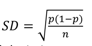
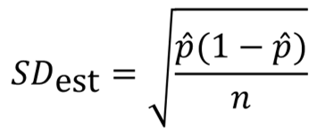
• For sample proportions, the standard deviation is $SD = \sqrt{\frac{p(1-p)}{n}}$

Conditions for the CLT

• Random, independent sample

• Large sample size (n is large enough)

• Population is much larger than the sample

Example: Estimating Probabilities with the CLT

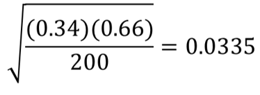
Suppose 34% of bacterial samples are antibiotic-resistant. In a random sample of 200, what is the probability that more than 40% are resistant?

• Check CLT conditions.

• Calculate standard deviation: $\sqrt{\frac{0.34 \times 0.66}{200}} = 0.0335$

• Convert to z-score and use the normal table to find the probability.

Summary

• Probability distributions model random events and are foundational in statistics.

• The normal and binomial distributions are key models for continuous and discrete data, respectively.

• Statistical inference allows us to draw conclusions about populations from samples, accounting for error and bias.

• The Central Limit Theorem explains why sample means and proportions are approximately normal for large samples, enabling probability calculations and hypothesis testing.