Lw Probability Models for Random Variables: Discrete and Continuous Distributions

Probability Models for Random Variables

Introduction to Random Variables

Random variables are fundamental in statistics for modeling outcomes of random phenomena. They can be classified as either discrete or continuous, depending on the set of possible values they can assume.

• Random Variable (X): A variable that takes on numerical values determined by the outcome of a random event.

• Notation: Capital letters (e.g., X) denote random variables; lowercase letters (e.g., x) denote specific values.

• Examples: The exact mass of a random animal (continuous), the year a student was born (discrete).

Types of Random Variables

• Discrete Random Variables: Take on a countable number of distinct values (e.g., number of accidents in a day).

• Continuous Random Variables: Can take any value within a range (e.g., size of fish in the sea).

Probability Distributions and Expected Value

Probability Distribution of a Random Variable

A probability distribution assigns probabilities to each possible value of a random variable. For discrete variables, this is a list or table; for continuous variables, it is a density curve.

• Expected Value (Mean, μ or E(X)): The long-run average value of the random variable over many repetitions.

Formula for Discrete Random Variables:

$\mu = E(X) = \sum x \cdot P(x)$

• Interpretation: The sum of each possible value multiplied by its probability.

• Practical meaning: The expected value is the average outcome if the random process is repeated many times.

Variance and Standard Deviation of a Random Variable

Variance and standard deviation measure the spread of a random variable's distribution.

• Variance (σ²): The expected squared deviation from the mean.

• Standard Deviation (σ): The square root of the variance.

$\sigma^2 = Var(X) = \sum (x - \mu)^2 \cdot P(x)$

$\sigma = SD(X) = \sqrt{Var(X)}$

Linear Transformations and Combinations of Random Variables

Adding or Multiplying by a Constant

• Adding a Constant (c): $E(X \pm c) = E(X) \pm c$; $Var(X \pm c) = Var(X)$

• Multiplying by a Constant (a): $E(aX) = aE(X)$; $Var(aX) = a^2 Var(X)$

Example: If everyone in a company receives a $5000 raise, the mean salary increases by $5000, but the variance does not change. If everyone receives a 10% raise, both the mean and variance increase (variance by the square of the multiplier).

Combining Random Variables

• Sum or Difference of Means: $E(X \pm Y) = E(X) \pm E(Y)$

• Variance of Sum or Difference (if independent): $Var(X \pm Y) = Var(X) + Var(Y)$

Example: If two couples each receive a random discount with mean $5.83 and SD $8.62, the combined mean is $11.66 and the combined SD is $17.24.

The Binomial Model and Bernoulli Trials

Bernoulli Trials

• Each trial has two possible outcomes: success or failure.

• The probability of success (p) is constant for each trial.

• Trials are independent.

The Binomial Model

The Binomial model describes the probability of observing a certain number of successes in a fixed number of independent Bernoulli trials.

• Parameters: n = number of trials, p = probability of success

• Notation: $X \sim Binom(n, p)$

Probability of Exactly k Successes:

$P(X = k) = {n \choose k} p^k (1-p)^{n-k}$

where ${n \choose k} = \frac{n!}{k!(n-k)!}$

• Mean: $\mu = np$

• Standard Deviation: $\sigma = \sqrt{np(1-p)}$

Critical Assumption: Independence

• Bernoulli trials must be independent. If sampling without replacement, the sample size should be less than 10% of the population (10% condition).

Example: Email Spam

• Suppose 91% of emails are spam. For 25 emails, let X = number of real messages.

• p = 0.09, n = 25, $X \sim Binom(25, 0.09)$

• Expected value: $E(X) = 25 \times 0.09 = 2.25$

• Standard deviation: $SD(X) = \sqrt{25 \times 0.09 \times 0.91} = 1.43$

• Probability of 1 or 2 real messages: $P(X=1) + P(X=2) = 0.2340 + 0.2777 = 0.5117$

Continuous Probability Models

The Uniform Model

• A continuous random variable X has a uniform distribution on (a, b) if its density is constant over that interval.

• Mean: $E(X) = \frac{a + b}{2}$

• Variance: $Var(X) = \frac{(b - a)^2}{12}$

• Probability for interval (c, d): $P(c < X < d) = \frac{d - c}{b - a}$

Example: Waiting for a train that comes every 10 minutes (a = 0, b = 10):

• Height of curve: $\frac{1}{b-a} = \frac{1}{10}$

• Average wait time: $E(X) = 5$ minutes

• Variance: $Var(X) = \frac{100}{12} \approx 8.33$

• Probability of waiting between 2 and 4 minutes: $\frac{4-2}{10-0} = 0.2$

The Normal Model

• The Normal distribution is a continuous model characterized by its mean (μ) and standard deviation (σ).

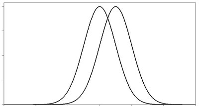
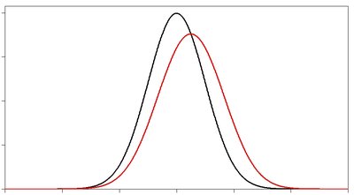
• Shifting or scaling a Normal random variable produces another Normal random variable with a new mean and/or standard deviation.

• The sum of independent Normal random variables is also Normal.

Approximating the Binomial with the Normal Model

• For large n, the Binomial distribution can be approximated by a Normal distribution with $\mu = np$ and $\sigma^2 = np(1-p)$, provided the Success/Failure Condition holds ($np \geq 10$ and $n(1-p) \geq 10$).

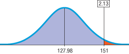
Example: Out of 1422 emails, 151 are real. Is this unusual if p = 0.09?

• $\mu = 1422 \times 0.09 = 127.98$

• $\sigma = \sqrt{1422 \times 0.09 \times 0.91} \approx 10.79$

• Standardized value: $z = \frac{151 - 127.98}{10.79} = 2.13$

• Probability $P(X \leq 151) = P(z \leq 2.13) = 0.9834$

Common Pitfalls and What Can Go Wrong

• Probability models are simplifications of reality; always check assumptions.

• Only add variances for independent random variables; do not add standard deviations directly.

• Do not use the Binomial model without verifying Bernoulli trial conditions.

• Do not use the Normal approximation for small n or when the Success/Failure Condition is not met.

• Not all distributions are Normal; check the context before applying the Normal model.

Summary of Key Formulas

• Expected Value (Discrete): $\mu = E(X) = \sum x \cdot P(x)$

• Variance (Discrete): $\sigma^2 = Var(X) = \sum (x - \mu)^2 \cdot P(x)$

• Standard Deviation: $\sigma = \sqrt{Var(X)}$

• Linear Transformations: $E(aX + c) = aE(X) + c$, $Var(aX + c) = a^2 Var(X)$

• Sum/Difference of Independent Variables: $E(X \pm Y) = E(X) \pm E(Y)$, $Var(X \pm Y) = Var(X) + Var(Y)$

• Binomial Probability: $P(X = k) = {n \choose k} p^k (1-p)^{n-k}$

• Normal Approximation: $\mu = np$, $\sigma^2 = np(1-p)$