Randomness and Probability: Foundations and Applications

Random Phenomena and Probability

Understanding Randomness

Random phenomena are situations in which individual outcomes are unpredictable, but the long-run behavior can be described probabilistically. Each attempt or trial produces an outcome, and an event refers to a single outcome or a combination of outcomes.

• Sample Space (S or Ω): The set of all possible outcomes.

• Probability of an Event: The long-run relative frequency of the event occurring.

• Independence: Two events are independent if the outcome of one does not affect the outcome of the other.

The Law of Large Numbers (LLN)

The LLN states that as the number of independent trials increases, the observed relative frequency of an event approaches its theoretical probability.

• Empirical Probability: Probability based on observed data from repeated trials.

The Nonexistent Law of Averages

Common Misconceptions

Many people mistakenly believe in a "Law of Averages," expecting that outcomes not seen in many trials are "due" to occur. This is incorrect; the probability of independent events does not change based on past outcomes.

Types of Probability

Model-Based (Theoretical) Probability

Theoretical probability is calculated based on models where all outcomes are equally likely.

• Formula: $P(A) = \frac{\text{Number of outcomes in } A}{\text{Total number of possible outcomes}}$

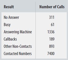
Example: In a survey of 10,190 randomly generated phone numbers, 7,400 resulted in contact. The probability of contact is $\frac{7400}{10190} = 0.7262$.

Personal (Subjective) Probability

Personal probability reflects an individual's degree of belief in an event, not based on long-run frequencies or equally likely outcomes.

Probability Rules

Basic Probability Rules

• Rule 1: $0 \leq P(A) \leq 1$ for any event A.

• Rule 2 (Probability Assignment Rule): $P(S) = 1$, where S is the sample space.

• Rule 3 (Complement Rule): $P(A^C) = 1 - P(A)$

Example: If 30% of customers make a purchase, the probability that a customer does not make a purchase is $1 - 0.30 = 0.70$.

Multiplication Rule for Independent Events

• Rule 4: For independent events A and B, $P(A \text{ and } B) = P(A) \times P(B)$

Example: Probability that two independent customers both make a purchase: $0.30 \times 0.30 = 0.09$.

Addition Rule for Disjoint Events

• Rule 5: For disjoint (mutually exclusive) events A and B, $P(A \text{ or } B) = P(A) + P(B)$

Example: Probability a customer makes a purchase in store (0.30) or online (0.09): $0.30 + 0.09 = 0.39$

Probability of no purchase: $1 - 0.39 = 0.61$

General Addition Rule

• Rule 6: For any events A and B, $P(A \text{ or } B) = P(A) + P(B) - P(A \text{ and } B)$

Example: Probability at least one of two customers makes a purchase: $0.30 + 0.30 - 0.20 = 0.40$

Comprehensive Example: Car Inspections

• P(Pass) = 0.75

• P(Not Pass) = 1 - 0.75 = 0.25

• P(Both Pass) = 0.75 \times 0.75 = 0.5625

• P(At least one passes) = 1 - (0.25)^2 = 0.9375

• P(Neither passes) = 1 - 0.9375 = 0.0625

Joint Probability and Contingency Tables

Contingency Tables

Contingency tables organize data for two or more categorical variables, showing joint and marginal probabilities.

• Marginal Probability: Probability based on totals in the margins (e.g., probability of being a woman).

• Joint Probability: Probability of two events occurring together (e.g., being a woman and choosing a camera).

• Conditional Probability: Probability of one event given another, $P(B|A)$.

Conditional Probability

• Definition: $P(B|A) = \frac{P(A \text{ and } B)}{P(A)}$

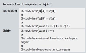
Events A and B are independent if $P(B|A) = P(B)$.

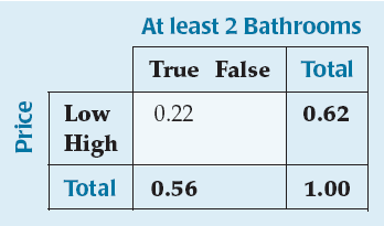
Example: Constructing a Contingency Table

A survey classifies homes by price and number of bathrooms. 56% have at least 2 bathrooms, 62% are low-priced, and 22% are both.

	True	False	Total
Low	0.22		0.62
High
Total	0.56		1.00

Example: Online Banking

Survey results: 30% bank online, 40% are under 50, 25% are under 50 and bank online.

	Yes	No	Total
Under 50	0.25	0.15	0.40
50 or Older	0.05	0.55	0.60
Total	0.30	0.70	1.00

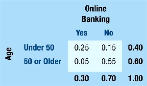
• Probability under 50 and banks online: $0.25 / 0.40 = 0.625$

• Banking online and age are not independent since $0.625 \neq 0.30$

Probability Trees

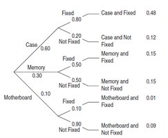
Tree Diagrams

Probability trees visually represent sequences of events and their probabilities, helping to calculate joint and conditional probabilities.

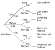
Joint probabilities at the ends of branches are found by multiplying probabilities along the path.

Reversing the Conditioning: Bayes’ Rule

Bayes’ Rule

Bayes’ Rule allows calculation of reverse conditional probabilities, especially when events are mutually exclusive and exhaustive.

• Formula: $P(A_i|B) = \frac{P(B|A_i)P(A_i)}{\sum_{j=1}^n P(B|A_j)P(A_j)}$

Common Pitfalls and Best Practices

• Probabilities must sum to 1 across all possible outcomes.

• Only add probabilities for disjoint events.

• Only multiply probabilities for independent events.

• Do not confuse disjoint and independent events.

Summary of Key Probability Rules

• Complement Rule: $P(A) = 1 - P(A^C)$

• Multiplication Rule (Independent): $P(A \text{ and } B) = P(A)P(B)$

• General Multiplication Rule: $P(A \text{ and } B) = P(A)P(B|A)$

• Addition Rule (Disjoint): $P(A \text{ or } B) = P(A) + P(B)$

• General Addition Rule: $P(A \text{ or } B) = P(A) + P(B) - P(A \text{ and } B)$

Constructing and Using Contingency Tables and Tree Diagrams

• Contingency tables help organize and analyze joint, marginal, and conditional probabilities.

• Tree diagrams are useful for visualizing sequences of events and calculating probabilities.

• Bayes’ Rule is essential for finding reverse conditional probabilities.