Real Applications of the Normal Distribution

Normal Probability Distributions

Introduction to the Normal Distribution

The normal distribution, also known as the Gaussian distribution, is one of the most important probability distributions in statistics. It is widely used because many real-world phenomena are approximately normally distributed. The distribution is named after the mathematician Johann Carl Friedrich Gauss.

• Symmetric bell-shaped curve: The normal distribution is perfectly symmetric about its mean.

• Unimodal: It has a single peak (mode).

• Mean, median, and mode are equal: All are located at the center of the distribution.

• Total area under the curve: Equals 1 (or 100%).

• Spread determined by standard deviation (σ): Larger σ means a wider, flatter curve.

• Notation: $X \sim N(\mu, \sigma)$, where $\mu$ is the mean and $\sigma$ is the standard deviation.

• Empirical Rule: The normal distribution follows the 68-95-99.7 rule for data within 1, 2, and 3 standard deviations from the mean.

The Normal Probability Density Function (PDF)

The probability density function (PDF) for a normal distribution is given by:

$f(x) = \frac{1}{\sigma \sqrt{2\pi}} e^{-\frac{1}{2} \left( \frac{x-\mu}{\sigma} \right)^2}$

However, in practice, probabilities are found using technology (such as calculators or software) rather than by direct calculation from the PDF.

The Standard Normal Distribution and Z-Scores

A standard normal distribution is a normal distribution with mean $\mu = 0$ and standard deviation $\sigma = 1$. The variable $Z$ is used to denote a standard normal random variable, written as $Z \sim N(0, 1)$. A z-score indicates how many standard deviations a value $x$ is from the mean:

$z = \frac{x - \mu}{\sigma}$

Probabilities for the standard normal distribution are found using $Z$-scores.

Applications of the Normal Distribution

Finding Probabilities Using Technology

Modern statistical practice uses technology (such as Desmos or statistical calculators) to find areas under the normal curve, which correspond to probabilities. The general format for finding probabilities in Desmos is:

• normaldist(mean, standard deviation) for the normal distribution

• Specify the region of interest (e.g., between two values, left of a value, right of a value)

Example 1: Proportion of Men Taller Than 72 Inches

Suppose heights of men are normally distributed with mean $\mu = 68.6$ in. and standard deviation $\sigma = 2.8$ in. What proportion of men are taller than 72 in.?

• Find $P(X \geq 72)$ using Desmos or similar technology.

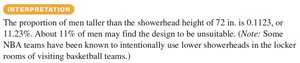
• Result: $P(X \geq 72) = 0.1123$ (or 11.23%)

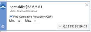
Interpretation: About 11% of men may find the showerhead design unsuitable if it is set at 72 inches.

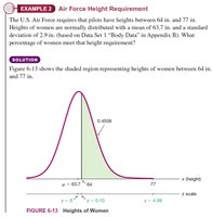
Example 2: Air Force Height Requirement

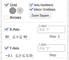
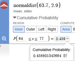
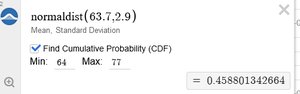
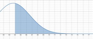
The U.S. Air Force requires that pilots have heights between 64 in. and 77 in. Heights of women are normally distributed with mean $\mu = 63.7$ in. and standard deviation $\sigma = 2.9$ in. What percentage of women meet this height requirement?

• Find $P(64 \leq X \leq 77)$ using technology.

• Result: $P(64 \leq X \leq 77) = 0.459$ (or 45.9%)

Finding Percentiles and Cutoff Values

Percentiles indicate the value below which a given percentage of observations fall. The inverse cumulative distribution function (inverse CDF) is used to find percentiles.

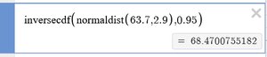
• Desmos format: inversecdf(normaldist(mean, std dev), percentile)

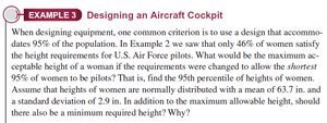
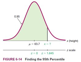
Example 3: Designing an Aircraft Cockpit

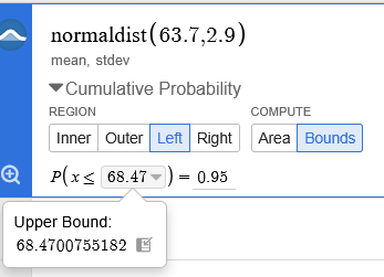
To accommodate the shortest 95% of women, find the 95th percentile of heights (mean $= 63.7$, standard deviation $= 2.9$).

• Find $x$ such that $P(X \leq x) = 0.95$

• Result: $x = 68.47$ in.

Identifying Significantly Low or High Values

Values that are in the extreme tails of the normal distribution (e.g., below the 5th percentile or above the 95th percentile) are considered significantly low or high.

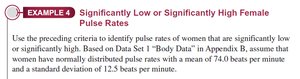
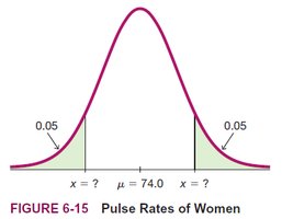
Example 4: Female Pulse Rates

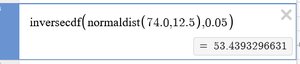
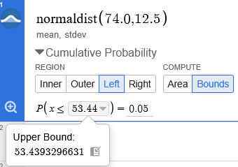
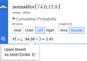
Assume women's pulse rates are normally distributed with mean $\mu = 74.0$ beats per minute and standard deviation $\sigma = 12.5$ beats per minute. Find the pulse rates that are significantly low (below the 5th percentile) and significantly high (above the 95th percentile).

• Low cutoff: $P(X \leq x) = 0.05$

• High cutoff: $P(X \leq x) = 0.95$

• Results: Low = 53.44 bpm, High = 94.56 bpm

Assessing Normality: Normal Probability Plots

Normal Quantile (Probability) Plots

A normal quantile plot (or normal probability plot) is used to assess whether a dataset is approximately normally distributed. The plot graphs each data value against its corresponding z-score.

• All points should lie roughly on a straight line if the data are normally distributed.

• No S-shaped pattern should be present.

• Outliers appear as points far from the overall pattern.

Example: Tylenol Weights (Bell-shaped)

Example: Electricity Data (Not Bell-shaped)

Summary Table: Properties of the Normal Distribution

Property	Description
Shape	Symmetric, bell-shaped
Center	Mean = Median = Mode
Spread	Determined by standard deviation ($\sigma$)
Total Area	1 (or 100%)
Notation	$X \sim N(\mu, \sigma)$
Empirical Rule	68-95-99.7% within 1, 2, 3 $\sigma$

Additional info: The use of technology such as Desmos streamlines the calculation of probabilities and percentiles for the normal distribution, making manual table lookups unnecessary in modern statistics courses.