Regression Diagnostics: Changing Variation, Outliers, and Dependent Errors

Regression Diagnostics

Introduction to Regression Diagnostics

Regression diagnostics are essential tools for evaluating the validity and reliability of regression models. They help identify issues such as changing variation (heteroscedasticity), outliers, and dependence among observations, which can undermine statistical inference and prediction accuracy.

Changing Variation in Regression Models

Understanding Changing Variation

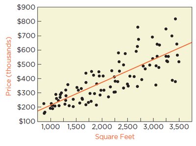
In regression analysis, the assumption of constant variance (homoscedasticity) of errors is crucial. When the variance of errors changes with the level of the explanatory variable, the data are said to exhibit heteroscedasticity. This can lead to unreliable confidence intervals and hypothesis tests.

• Homoscedasticity: Errors have equal variance across all levels of the explanatory variable.

• Heteroscedasticity: Errors have different variances, often increasing or decreasing with the explanatory variable.

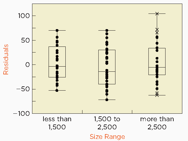
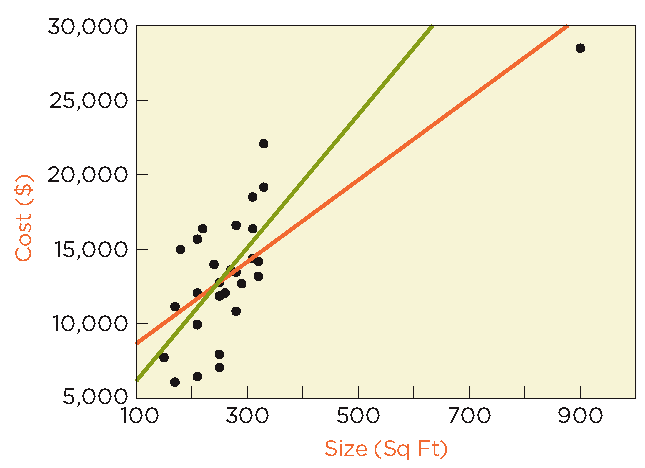
Example: Home prices tend to be more variable for larger homes, leading to heteroscedasticity in a regression of price on home size.

Detecting Changing Variation

Several graphical and statistical methods can be used to detect changing variation:

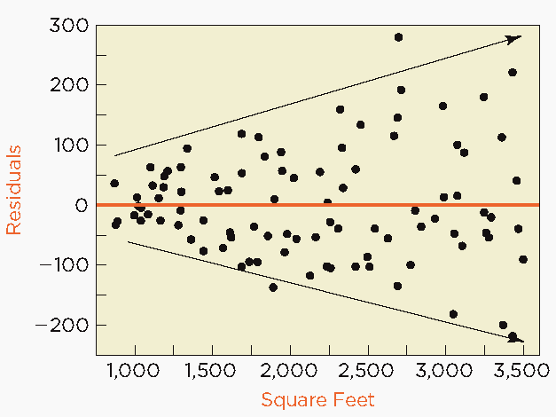
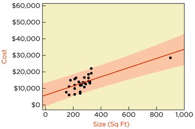
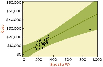
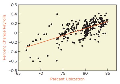
• Residual Plots: A fan-shaped pattern in a plot of residuals versus fitted values or explanatory variable indicates heteroscedasticity.

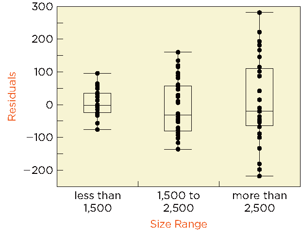
• Side-by-Side Boxplots: Comparing the spread of residuals across groups of the explanatory variable can reveal differences in variance.

Consequences of Heteroscedasticity

• Prediction intervals may be too narrow or too wide, depending on the value of the explanatory variable.

• Confidence intervals for regression coefficients (slope and intercept) are unreliable.

• Hypothesis tests for coefficients may not be valid.

Fixing Heteroscedasticity: Model Revision

One common remedy is to transform the response and/or explanatory variable to stabilize variance. For example, dividing both sides of the regression equation by the explanatory variable can yield a model with more constant variance:

• Let Price = F + M × SqFt + ε (original model)

• Divide both sides by SqFt: $\text{Price/SqFt} = F/\text{SqFt} + M + \varepsilon'$

• Now, regress Price per SqFt on 1/SqFt.

This transformation often results in residuals with similar variances (homoscedasticity).

Comparing Models: Original vs. Transformed

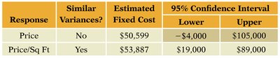
Although the transformed model may have a lower $r^2$, it provides more reliable confidence and prediction intervals.

Response	Similar Variances?	Estimated Fixed Cost	95% Confidence Interval
Price	No	$50,599	−$4,000 to $105,000
Price/Sq Ft	Yes	$53,887	$19,000 to $89,000

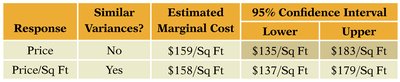
Response	Similar Variances?	Estimated Marginal Cost	95% Confidence Interval
Price	No	$159/Sq Ft	$135 to $183/Sq Ft
Price/Sq Ft	Yes	$158/Sq Ft	$137 to $179/Sq Ft

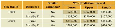
Size (Sq Ft)	Response	Similar Variances?	95% Prediction Interval Lower	Upper	Length
1,000	Price	No	$28,000	$392,000	$364,000
1,000	Price/Sq Ft	Yes	$133,000	$290,000	$157,000
3,000	Price	No	$347,000	$711,000	$364,000
3,000	Price/Sq Ft	Yes	$291,000	$765,000	$474,000

Outliers in Regression

Identifying and Understanding Outliers

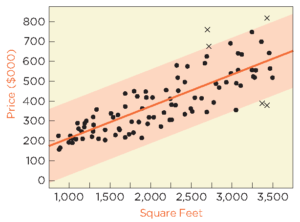
An outlier is an observation that deviates markedly from other observations. In regression, an outlier can have a large influence on the fitted line, especially if it is a leveraged observation (i.e., has an extreme value of the explanatory variable).

• Leveraged Observation: An observation with an unusually high or low value of the explanatory variable, which can pull the regression line toward itself.

Consequences of Outliers

Outliers can significantly affect regression estimates:

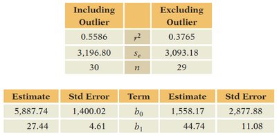
• Including an outlier can shift the estimated intercept and slope by more than one standard error.

• Prediction intervals can change substantially depending on whether the outlier is included.

	Including Outlier	Excluding Outlier
$r^2$	0.5586	0.3765
$s_e$	3,196.80	3,093.18
n	30	29

Term	Estimate (Incl.)	Std Error (Incl.)	Estimate (Excl.)	Std Error (Excl.)
$b_0$	5,887.74	1,400.02	1,558.17	2,877.88
$b_1$	27.44	4.61	44.74	11.08

Handling Outliers

• If the outlier is representative of future data, it should be included in the analysis.

• If the outlier is due to error or is not representative, it may be excluded, but justification is needed.

Dependent Errors and Time Series

Detecting Dependence in Errors

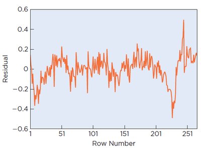
In time series data, errors may be correlated across time (autocorrelation), violating the independence assumption of regression. This can be detected by plotting residuals versus time and using statistical tests such as the Durbin-Watson statistic.

• Autocorrelation: Correlation between adjacent residuals in time series data.

• Durbin-Watson Statistic: Tests the null hypothesis $H_0: \rho_\varepsilon = 0$ (no autocorrelation).

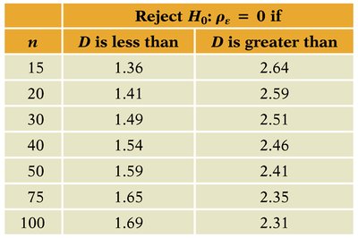
Durbin-Watson Statistic

The Durbin-Watson statistic is calculated as:

$D = \frac{\sum_{i=2}^n (e_i - e_{i-1})^2}{\sum_{i=1}^n e_i^2}$

Critical values depend on sample size. If $D$ is much less than 2, positive autocorrelation is indicated.

n	D is less than	D is greater than
15	1.36	2.64
20	1.41	2.59
30	1.49	2.51
40	1.54	2.46
50	1.59	2.41
75	1.65	2.35
100	1.69	2.31

Consequences and Remedies for Dependent Errors

• Standard errors are underestimated, making confidence intervals and hypothesis tests unreliable.

• Regression coefficients are less precise than indicated.

• Best remedy: Incorporate dependence structure into the model (e.g., use time series models).

Case Study: Predicting Cell Phone Subscribers

Application of Regression Diagnostics

Simple regression can be used to predict the number of cell phone subscribers over time. However, if residuals show autocorrelation, statistical inferences are not reliable.

• Regression equation: $\text{Estimated Subscribers} = -40,142 + 20.1 \times \text{Date}$

• Timeplot of residuals and Durbin-Watson statistic indicate violation of independence.

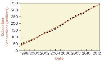
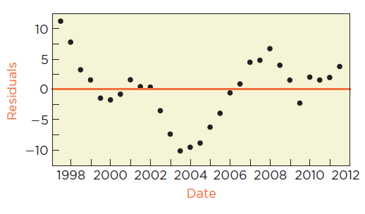
Conclusion: While the regression shows a strong upward trend, the violation of model assumptions means that prediction intervals and statistical inferences are not trustworthy.