Regression Diagnostics, Residual Analysis, and Model Assumptions in Linear Regression

Regression Analysis and Diagnostics

Analysis of Variance (ANOVA) in Regression

ANOVA is used in regression to partition the total variation in the response variable into components explained by the model and those due to error. This helps assess the effectiveness of the regression model.

• Signal: Variation explained by the linear model.

• Noise: Variation from residuals (errors).

• Total Variation: The sum of signal and noise, representing the total variation in the response variable.

• Sum of Squares (SS): Measures the variation for each component.

ANOVA Table:

Source of Variation	SS	df
Regression	$SSR = \sum (\hat{Y}_i - \bar{Y})^2$	1
Error	$SSE = \sum (Y_i - \hat{Y}_i)^2$	n - 2
Total	$SSTO = \sum (Y_i - \bar{Y})^2$	n - 1

Relationship Between $R^2$ and Standard Error ($s_e$)

$R^2$ measures the proportion of variance explained by the model, while $s_e$ is the standard deviation of the residuals. As $R^2$ increases, $s_e$ typically decreases, indicating a better fit.

• $R^2$: $R^2 = 1 - \frac{SSE}{SSTO}$

• Standard Error of Residuals ($s_e$): $s_e = \sqrt{\frac{SSE}{n-2}}$

• Interpretation: Lower $s_e$ means predictions are closer to actual values.

Comparing Standard Deviations

Comparing the standard deviation of the response variable ($s_y$) and the standard error of the residuals ($s_e$) helps assess model quality.

• $s_y$: Standard deviation of the response variable.

• $s_e$: Standard deviation of residuals.

• Interpretation: If $s_e < s_y$, the model improves prediction.

Regression Assumptions and Conditions

Conditions for Least Squares Regression

To ensure valid regression results, several conditions must be checked:

• Quantitative Variable Condition: Both variables must be quantitative.

• Straight Line Condition: The relationship should be linear, as seen in scatterplots and residual plots.

• Outlier Condition: Outliers can distort the regression line; problematic outliers should be addressed.

• Equal Spread Condition: The spread of residuals should be consistent across values of the explanatory variable (no fanning).

• Independence: Residuals should be independent, especially important for time series data.

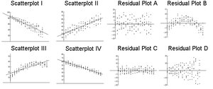
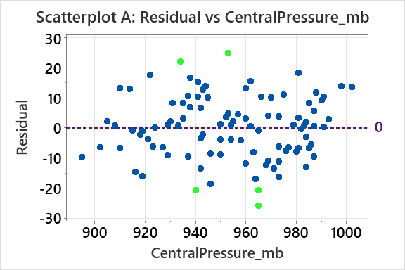
Scatterplots and Residual Plots

Matching scatterplots to residual plots helps diagnose model fit and violations of assumptions.

• Scatterplot: Shows the relationship between variables.

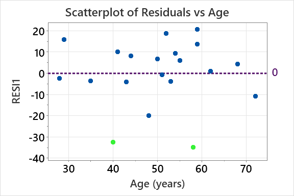
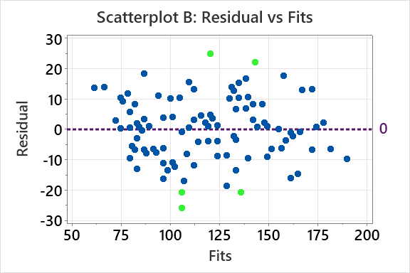
• Residual Plot: Plots residuals against explanatory variable or fits to check for patterns.

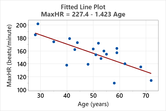
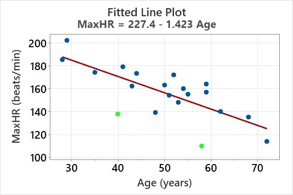
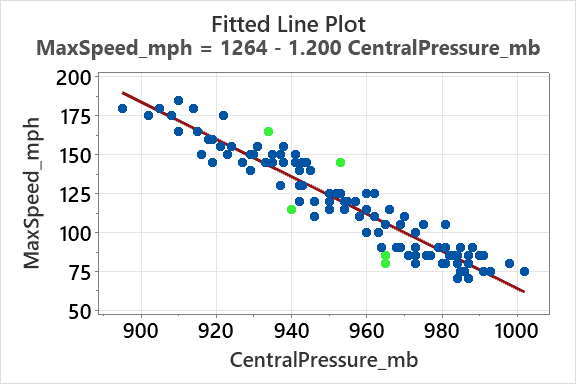
Example: Fitted Line Plot and Outliers

Regression models can be visualized with fitted line plots. Outliers are points that deviate significantly from the fitted line.

• Fitted Line Equation: $\text{MaxHR} = 227.4 - 1.423 \times \text{Age}$

• Outliers: Points far from the line may be flagged as unusual.

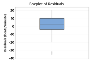
Residual Analysis

Residuals are the differences between observed and predicted values. Analyzing residuals helps identify outliers and assess model assumptions.

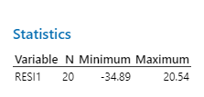
• Boxplot of Residuals: Visualizes the spread and identifies extreme values.

• Statistics: Minimum and maximum residuals indicate the range.

Flagging Unusual Observations

Statistical software (e.g., Minitab) flags observations with large residuals (R flag) or high leverage (X flag).

• R Flag: Standardized residual $> 2.0$ (in absolute value).

• X Flag: High leverage, far from mean of explanatory variable.

Regression Model Refinement and Outlier Impact

Impact of Removing Outliers

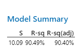
Removing flagged outliers can affect model coefficients, $R^2$, and $s_e$. Comparing model summaries before and after removal helps assess impact.

• Model Summary: Shows $s_e$ and $R^2$ values.

• Interpretation: Little change suggests outliers are not problematic.

Residual Plots for Model Diagnostics

Residual plots against explanatory variables and fits help detect patterns such as fanning or thickening, which violate equal spread condition.

Prediction and Extrapolation

Making Predictions with Regression Models

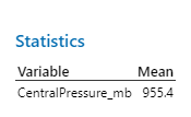
Regression models can predict values of the response variable for given values of the explanatory variable. Predictions are most trustworthy near the mean of the explanatory variable.

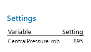
• Extrapolation: Predicting beyond the range of observed data is risky and often unreliable.

• Prediction Example: For Central Pressure values of 940, 955.4, and 970 millibars, predicted MaxSpeed can be calculated using the regression equation.

Outliers, Leverage, and Influence

Leverage and Influential Observations

Leverage measures how far an observation's explanatory variable is from the mean. Highly influential observations can greatly affect model coefficients.

• Leverage: High leverage points have x-values far from the mean.

• Influence: Highly influential points change the regression line significantly when removed.

Anscombe's Quartet and Model Diagnostics

Anscombe's Quartet demonstrates that datasets with similar statistical properties can have very different distributions and regression fits. Visual inspection is crucial.

• R-squared: $R^2 = (r)^2 = (0.816)^2 = 0.67$ or 67%

• Graphical Analysis: Each dataset shows different patterns, outliers, and influential points.

Final Tips: Regression Diagnostics

Summary of Diagnostic Flags

• Large Outliers (R Flag): Increase $s_e$, decrease $R^2$.

• High Leverage (X Flag): Lead to imprecise predictions.

• Highly Influential Observations: Greatly change model coefficients when removed; may have X or RX flags.

Key Formulas

• Regression Equation: $y = \beta_0 + \beta_1 x$

• Residual: $e_i = y_i - \hat{y}_i$

• Standardized Residual: $e_i^* = \frac{e_i}{s_e}$

• R-squared: $R^2 = 1 - \frac{SSE}{SSTO}$

Example Table: Diagnostic Flags

Obs	MaxSpeed_mph	Fit	Resid	Std Resid	Flag
46	180.00	189.90	-9.90	-1.01	X
68	80.00	105.89	-25.89	-2.58	R
70	115.00	135.90	-20.90	-2.08	R
74	85.00	105.89	-20.89	-2.08	R
79	165.00	143.10	21.90	2.19	R
100	145.00	120.29	24.71	2.46	R

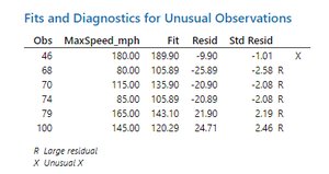
Example: In hurricane data, points with large residuals or high leverage are flagged, and their impact on the regression model is assessed.

Conclusion

Regression diagnostics are essential for validating model assumptions, identifying outliers, and ensuring reliable predictions. Visual tools and statistical flags help guide model refinement and interpretation.