Relationships Between Categorical Variables: Contingency Tables and Graphical Displays

Relationships Between Categorical Variables

Introduction

Understanding the relationship between two categorical variables is a fundamental aspect of introductory statistics. This chapter explores how to summarize and visualize such relationships using contingency tables and various graphical displays.

Types of Bivariate Categorical Data Displays

• Contingency Tables

• Side by Side Pie Charts

• Segmented Bar Charts

• Mosaic Plots

Contingency Tables

Definition and Structure

A contingency table (also called a two-way table) is a tabular summary that displays the frequency distribution of variables. It allows us to examine the relationship between two categorical variables by showing the counts for each combination of categories.

• Rows typically represent categories of one variable.

• Columns represent categories of the second variable.

• Cells contain the count (frequency) for each combination.

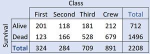
Example: The table below shows the relationship between Survival (Alive/Dead) and Class (First, Second, Third, Crew) for Titanic passengers.

Marginal Distributions

The marginal distribution of a variable is the distribution of values for that variable alone, found in the margins (totals) of the contingency table.

• Row totals give the marginal distribution for the row variable.

• Column totals give the marginal distribution for the column variable.

Example: The marginal distribution of Survival (Alive/Dead) and Class (First, Second, Third, Crew) can be read from the totals in the table above.

Conditional Distributions

Definition and Calculation

A conditional distribution shows the distribution of one variable for individuals who satisfy a specific condition on another variable. It is calculated by focusing on a single row or column and dividing each cell count by the total for that row or column.

• Conditional on a row: Divide each cell in the row by the row total.

• Conditional on a column: Divide each cell in the column by the column total.

Example: The conditional distribution of Survival, given that a person was a crew member:

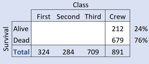
Here, 24% of crew survived and 76% died.

Example: The conditional distribution of Class, given that a person survived:

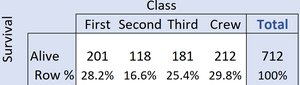
Among survivors, 28.2% were in First Class, 16.6% in Second, 25.4% in Third, and 29.8% were Crew.

Example: The conditional distribution of Class, given that a person died:

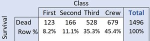
Among those who died, 8.2% were in First Class, 11.1% in Second, 35.3% in Third, and 45.4% were Crew.

Interpreting Conditional Distributions

• If the conditional distributions of one variable are the same across all categories of the other variable, the variables are independent.

• If the conditional distributions differ, the variables are associated (not independent).

Graphical Displays for Categorical Data

Side by Side Pie Charts

Side by side pie charts visually compare the conditional distributions of a categorical variable across the categories of another variable. Each pie chart represents a different group (e.g., survivors vs. non-survivors), and the slices show the proportion in each category (e.g., class).

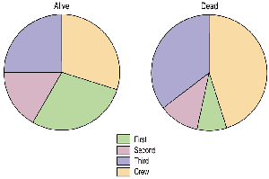
These charts show that the distribution of Class differs between those who survived and those who did not, suggesting an association between Class and Survival.

Segmented Bar Charts

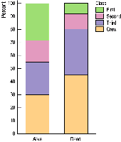
A segmented bar chart (also called a stacked bar chart) displays the same information as side by side pie charts, but uses bars divided into segments proportional to the frequencies or percentages in each category.

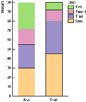
This chart makes it easy to compare proportions across groups and see differences in distributions.

Mosaic Plots

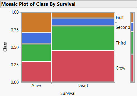
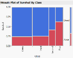
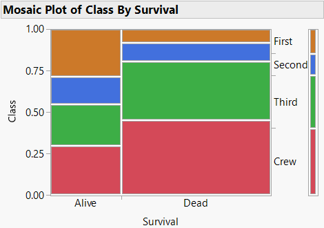
A mosaic plot is a graphical display that shows the relationship between two categorical variables. The width of each bar is proportional to the frequency of the category on the horizontal axis, and the height of each segment is proportional to the conditional frequency of the category on the vertical axis.

In the Titanic example, the mosaic plot shows that 32% survived and 68% died, with the distribution of class varying between survivors and non-survivors.

Segmented Bar Chart vs. Mosaic Plot

Both segmented bar charts and mosaic plots display conditional distributions, but mosaic plots also encode the marginal distribution by varying the width of the bars. This can make it easier to see both the overall and conditional relationships.

Choice of X and Y Variables

When creating contingency tables and mosaic plots, the choice of which variable is on the horizontal (X) or vertical (Y) axis can affect the visual interpretation, but not the underlying association. Sometimes, one arrangement makes patterns more apparent.

Another Example: Classroom Seating and Gender

Survey Data

Suppose 100 randomly selected students are surveyed about their gender (0 = female, 1 = male) and where they prefer to sit in a classroom (1 = front, 2 = middle, 3 = back, 4 = no preference).

To analyze the relationship, calculate the percentage of females and males who prefer to sit near the back. If the percentages differ, this suggests an association between gender and seating preference.

Mosaic Plot Example

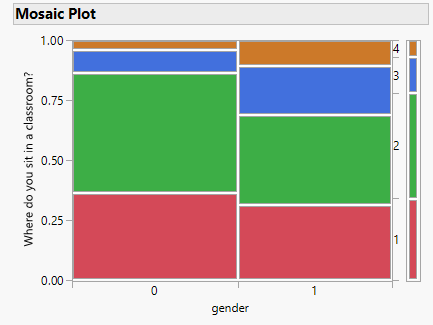
This mosaic plot visually displays the relationship between gender and seating preference, allowing for easy comparison of distributions.

Summary Table: Types of Graphical Displays for Categorical Data

Display Type	Main Purpose	Key Features
Contingency Table	Summarize counts for combinations of two categorical variables	Shows frequencies and marginal totals
Side by Side Pie Charts	Compare conditional distributions visually	Each pie represents a group; slices show proportions
Segmented Bar Chart	Compare conditional distributions visually	Bars divided into segments proportional to category frequencies
Mosaic Plot	Show both marginal and conditional distributions	Bar widths and heights proportional to frequencies

Key Terms and Concepts

• Contingency Table: A table showing the frequency distribution for two categorical variables.

• Marginal Distribution: The distribution of a single variable in a contingency table, found in the margins.

• Conditional Distribution: The distribution of one variable for individuals who satisfy a condition on another variable.

• Independence: Two variables are independent if the conditional distribution of one variable is the same for all categories of the other variable.

• Association: Two variables are associated if the conditional distributions differ.

Formulas

• Conditional Probability: The probability of event A given event B is $P(A \mid B) = \frac{P(A \cap B)}{P(B)}$

• Row Percentage (Conditional on Row): $\text{Row Percentage} = \frac{\text{Cell Count}}{\text{Row Total}} \times 100$

• Column Percentage (Conditional on Column): $\text{Column Percentage} = \frac{\text{Cell Count}}{\text{Column Total}} \times 100$