Review of Confidence Intervals and Basic Statistical Inference

Review of Basic Statistics

Why Learn Statistics?

Statistics is the discipline that transforms raw information into meaningful insights, enabling informed decision-making and action. It is foundational for understanding data in various fields, from science to business.

• Descriptive Statistics: Summarizes and describes the main features of a dataset.

• Graphical Summaries: Common visualizations include pie charts, bar graphs, histograms, and scatterplots.

• Numerical Summaries: Key measures include:

  • Measures of Central Tendency: Mean, median, and mode.

  • Measures of Dispersion: Range, variance, and standard deviation.

Statistical Inference

Introduction to Statistical Inference

Statistical inference involves using sample data (statistics) to make conclusions about a larger population (parameters). This process is essential for making predictions and testing hypotheses.

• Population: The entire group of interest.

• Sample: A subset of the population used for analysis.

• Parameter: A numerical summary of a population.

• Statistic/Estimate: A numerical summary of a sample.

• Sampling Designs: Includes simple random sampling and stratified random sampling.

• Observational Studies vs. Randomized Controlled Experiments: Observational studies observe without intervention, while experiments assign treatments to study effects.

• Association is not causation: Correlation does not imply a causal relationship.

• Treatment Group vs. Control Group: Used in experiments to compare outcomes.

Sampling Distributions & Confidence Intervals

Distribution of Sample Proportion

For a simple random sample of size n with population proportion p, the sampling distribution of the sample proportion \( \hat{p} \) is approximately normal if certain conditions are met.

• Shape: Approximately normal if \( np(1-p) \geq 10 \).

• Mean: \( \mu_{\hat{p}} = p \)

• Standard Deviation: \( \sigma_{\hat{p}} = \sqrt{\frac{p(1-p)}{n}} \)

Distribution of Sample Mean

The sampling distribution of the sample mean \( \bar{x} \) depends on the population distribution and sample size.

• If the population is normal: The sample mean is normally distributed for any sample size.

• If the population is not normal: The sample mean becomes approximately normal as the sample size increases (Central Limit Theorem).

• Mean: \( \mu_{\bar{x}} = \mu \)

• Standard Deviation: \( \sigma_{\bar{x}} = \frac{\sigma}{\sqrt{n}} \)

Point Estimates and Confidence Intervals

Key Concepts

• Point Estimate: A single value estimate of a population parameter (e.g., sample mean \( \bar{x} \)).

• Confidence Interval (CI): A range of values, derived from the sample, that is likely to contain the population parameter.

• Level of Confidence: The probability that the CI contains the true parameter (commonly 95%).

• Margin of Error: The maximum expected difference between the true parameter and a sample estimate.

• Critical Value: The value from the standard normal (z) or t-distribution corresponding to the desired confidence level.

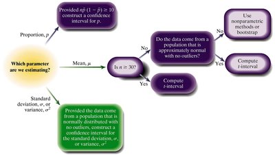
Choosing the Appropriate Confidence Interval

The type of confidence interval depends on the variable of interest and the data type.

• Population Proportion: Use when data are qualitative with two possible outcomes (e.g., Yes/No).

• Population Mean: Use when data are quantitative and summarized by mean and standard deviation.

Conditions for Constructing Confidence Intervals

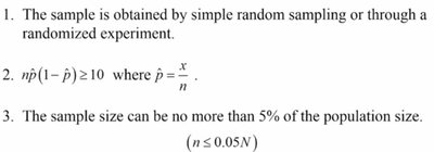
For a Population Proportion

• The sample is obtained by simple random sampling or a randomized experiment.

• \( np(1-\hat{p}) \geq 10 \), where \( \hat{p} = \frac{x}{n} \).

• The sample size is no more than 5% of the population size (\( n \leq 0.05N \)).

For a Population Mean

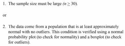
• The sample must be obtained by simple random sampling or a randomized experiment, and \( n \leq 0.05N \).

• Either:

  • The sample size is large (\( n \geq 30 \)), or

  • The data come from a population that is at least approximately normal with no outliers (verified using a normal probability plot and a boxplot).

Formulas for Confidence Intervals

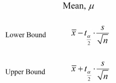
For a Population Mean (\( \mu \))

• Lower Bound: $\bar{x} - t_{\alpha/2} \cdot \frac{s}{\sqrt{n}}$

• Upper Bound: $\bar{x} + t_{\alpha/2} \cdot \frac{s}{\sqrt{n}}$

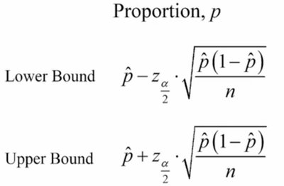
For a Population Proportion (\( p \))

• Lower Bound: $\hat{p} - z_{\alpha/2} \cdot \sqrt{\frac{\hat{p}(1-\hat{p})}{n}}$

• Upper Bound: $\hat{p} + z_{\alpha/2} \cdot \sqrt{\frac{\hat{p}(1-\hat{p})}{n}}$

Examples and Applications

Example: Constructing a Confidence Interval for a Mean

Suppose Robert wishes to estimate the mean number of miles his car can be driven on a full tank of gas. He collects a random sample of 10 measurements:

• Sample mean (\( \bar{x} \)): 380.67

• Sample standard deviation (s): 42.47

• Sample size (n): 10

To construct a 95% confidence interval, verify normality and absence of outliers using a boxplot and a normal probability plot.

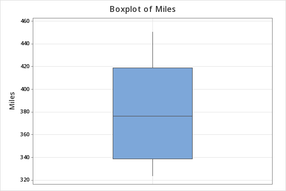
The boxplot shows no outliers, supporting the assumption of normality.

Using the t-distribution with 9 degrees of freedom (n-1), the critical value \( t_{0.025} = 2.262 \).

• Lower Bound: $380.67 - 2.262 \cdot \frac{42.47}{\sqrt{10}} = 350.29$

• Upper Bound: $380.67 + 2.262 \cdot \frac{42.47}{\sqrt{10}} = 411.05$

Interpretation: We are 95% confident that the population mean miles driven on a full tank of gas is between 350.29 and 411.05.

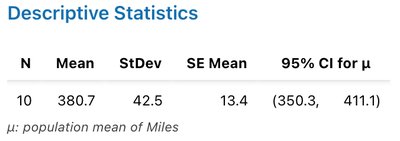
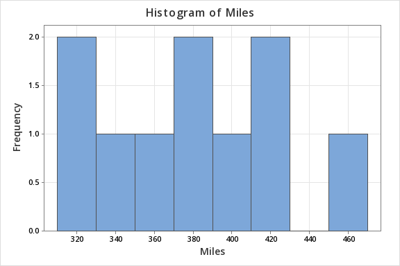
Summary Table: Descriptive Statistics for Miles Driven

Variable	N	Mean	SE Mean	StDev	Minimum	Q1	Median	Q3	Maximum
Miles	10	380.67	13.43	42.47	323.9	339.025	376.65	419.075	450.7

Practice: Identifying the Appropriate Confidence Interval

• Quantitative variable (e.g., time spent studying): Use a confidence interval for the mean.

• Qualitative variable with two outcomes (e.g., Yes/No): Use a confidence interval for the proportion.

Additional info: The examples provided reinforce the importance of matching the confidence interval method to the type of variable and data collected.