Sampling and Statistical Inference: Core Concepts for Introductory Statistics

Sampling and Statistical Inference

Introduction to Sampling and Inference

Sampling and statistical inference are foundational concepts in statistics, allowing us to draw conclusions about a population based on information from a sample. This section introduces the logic and methods for making inferences about population means and proportions, emphasizing the inherent uncertainty in such estimates.

• Population Mean: The average value of a variable for the entire population (e.g., average annual purchases per customer).

• Population Percent (Proportion): The fraction or percent of the population with a certain characteristic (e.g., unemployment rate).

• Sample: A subset of the population, used when it is impractical or impossible to collect data from the entire population.

• Statistical Inference: The process of using sample data to estimate and draw conclusions about population parameters, while quantifying uncertainty.

Key Point: Sampling is essential when full population data is unavailable, and statistical inference provides tools to estimate population values and measure the reliability of these estimates.

Sampling Error and Types of Inference

Sampling Error

Sampling error arises because the sample mean or proportion may differ from the true population value due to random variation. Even a representative sample provides only an imperfect estimate of the population parameter.

• Sampling Error: The difference between the sample statistic and the population parameter caused by the randomness of which individuals are included in the sample.

Types of Statistical Inference

There are three main types of inference you can make from a sample:

1. Estimation: Using the sample mean or proportion as the best estimate of the population value.

2. Confidence Interval: Providing a range of values within which the population parameter is likely to fall, with a specified level of confidence (e.g., 95%).

3. Test of Significance (Hypothesis Test): Assessing whether the population parameter is likely to be above or below a critical value of interest.

Example: If a sample of 100 customers has an average planned expenditure of $32.51, you might estimate the population mean as $32.51, construct a 95% confidence interval (e.g., $27.37 to $37.65), or test whether the mean exceeds a breakeven value (e.g., $27).

Estimation and Confidence Intervals

Constructing Confidence Intervals

A confidence interval quantifies the uncertainty in your estimate of the population mean or proportion. The width of the interval depends on the sample size (n) and the sample standard deviation (s).

• Sample Mean (m): The average of the sample values.

• Sample Standard Deviation (s): Measures the spread of sample values.

• Standard Error (SE): The estimated standard deviation of the sample mean, calculated as $s / \sqrt{n}$.

The confidence interval for the population mean is constructed as follows:

• 68% Confidence Interval: $m \pm s / \sqrt{n}$

• 95% Confidence Interval: $m \pm 2s / \sqrt{n}$

• 99.7% Confidence Interval: $m \pm 3s / \sqrt{n}$

Key Point: The confidence interval depends on the absolute sample size, not the percentage of the population sampled.

Example: For a sample mean $m = 32.51$, $s = 25.7$, $n = 100$:

• Standard error: $25.7 / 10 = 2.57$

• 68% CI: $32.51 \pm 2.57 = [29.94, 35.08]$

• 95% CI: $32.51 \pm 2 \times 2.57 = [27.37, 37.65]$

• 99.7% CI: $32.51 \pm 3 \times 2.57 = [24.80, 40.22]$

Statistical Significance and the t-Statistic

Testing Statistical Significance

Statistical significance tests determine whether the population parameter is likely to be above or below a critical value (c), such as a breakeven point.

• t-Statistic: $t = \frac{m - c}{s / \sqrt{n}}$

• If $|t| > 2$, the result is significant at the 2.5% level (outside the 95% confidence interval).

• If $|t| > 3$, the result is significant at the 0.15% level (outside the 99.7% confidence interval).

Significance vs. Importance: A statistically significant result may not be practically important, especially with large samples. Always consider the context and practical implications.

Sample Size Determination

The required sample size depends on the desired confidence interval length (L) and confidence level. The formulas are:

• For 68% confidence: $n = 4s^2 / L^2$

• For 95% confidence: $n = 16s^2 / L^2$

• For 99.7% confidence: $n = 36s^2 / L^2$

Example: If $s = 25.7$ and $L = 2$, then for 95% confidence, $n = 2,642$.

Inference for Population Proportions

Estimating Population Proportions

Inference for population proportions (percents) follows the same logic as for means. Each observation is coded as 0 or 1, and the sample proportion (f) is the mean of these values.

• Sample Proportion (f): Fraction of 1's in the sample.

• Sample Standard Deviation (s): $s = \sqrt{f(1-f) \cdot n/(n-1)}$ (for large n, $s \approx \sqrt{f(1-f)}$)

• Standard Error: $s / \sqrt{n}$

Example: In a sample of 100 voters, 52 support candidate X ($f = 0.52$):

• $s = \sqrt{0.52 \times 0.48} = 0.4996$

• Standard error: $0.4996 / 10 = 0.04996$

• 95% CI: $0.52 \pm 2 \times 0.04996 = [0.4201, 0.6199]$

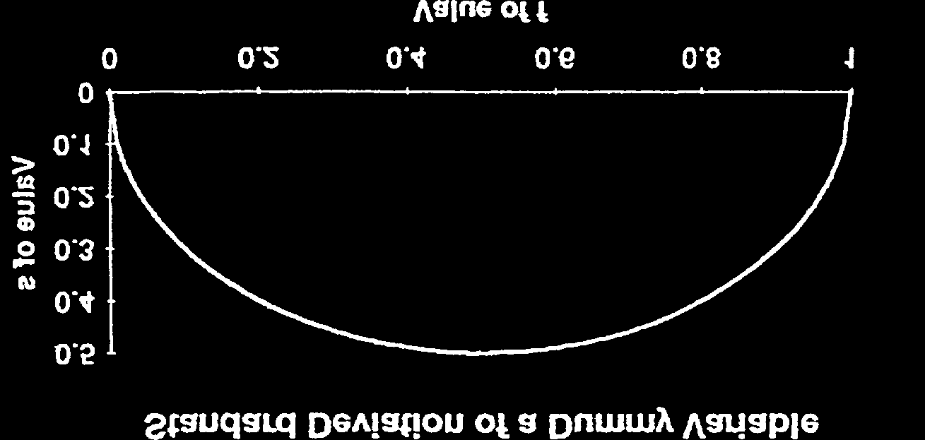
Key Point: For proportions, the maximum standard deviation occurs when $f = 0.5$.

Sources of Error Beyond Sampling

Response Bias

Response bias occurs when survey respondents do not provide accurate answers, due to changing opinions, misunderstanding questions, or the influence of question wording.

• Example: Different wording of survey questions about advertising can yield very different results.

Representativeness and Random Sampling

A sample should be representative of the population. The best way to ensure this is through random sampling, where every member of the population has an equal chance of selection. In practice, true random samples are difficult to obtain due to nonresponse and practical limitations.

• Random Sample: Every member of the population has an equal chance of being selected.

• Nonresponse: Some selected individuals do not participate, potentially biasing results.

• Corrective Actions: Replacing nonrespondents with demographically similar individuals can help, but may not fully eliminate bias.

Appendix: Key Formulas and Computations

Sample Mean and Standard Deviation

• Sample Mean (m): $m = \frac{1}{n} \sum_{i=1}^n x_i$

• Sample Standard Deviation (s): $s = \sqrt{\frac{1}{n-1} \sum_{i=1}^n (x_i - m)^2}$

• For dummy variables: $s = \sqrt{f(1-f) \cdot n/(n-1)}$

Standard Error

• Standard Error: $s / \sqrt{n}$

Finite Population Correction (fpc)

• When sampling without replacement from a finite population of size N:

• Corrected Standard Error: $s \sqrt{\frac{N-n}{N-1}} / \sqrt{n}$

• For large populations (n < 10% of N), the correction is negligible.

Summary Table: Key Formulas

Concept	Formula
Sample Mean (m)	$m = \frac{1}{n} \sum_{i=1}^n x_i$
Sample Standard Deviation (s)	$s = \sqrt{\frac{1}{n-1} \sum_{i=1}^n (x_i - m)^2}$
Standard Error (SE)	$s / \sqrt{n}$
Confidence Interval (95%)	$m \pm 2s / \sqrt{n}$
t-Statistic	$t = \frac{m - c}{s / \sqrt{n}}$
Sample Size (95% CI, length L)	$n = 16s^2 / L^2$

Additional info: The notes also introduce the concept of degrees of freedom (n-1 for sample standard deviation) and discuss the finite population correction for standard error, which is generally negligible unless the sample is a large fraction of the population.