Sampling Distribution Models and Confidence Intervals for Proportions

Sampling Distribution Models and Confidence Intervals for Proportions

Statistical Inference and Data Collection

Statistical inference is the process of using data collected from a sample to make conclusions about a population. The cycle of statistics involves collecting data, describing and displaying it, comparing groups, and making inferences about the population using probability models.

• Population: The entire group we want to learn about.

• Sample: A subset of the population selected for study.

• Statistical Inference: Using probability to estimate population parameters based on sample statistics.

• Sampling Error/Variability: The natural variation in sample statistics from one sample to another.

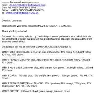
Example: Estimating the proportion of blue M&Ms in a bag by taking a random sample and calculating the observed proportion.

Sampling Distribution for Proportions

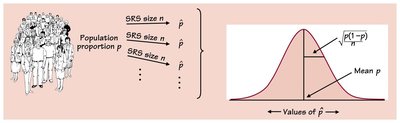
The sampling distribution is the distribution of a statistic (such as sample proportion) calculated from all possible samples of a given size from the same population. It allows us to understand how sample statistics vary and to quantify uncertainty in our estimates.

• Sampling Distribution: The distribution of values of a statistic from all possible samples of the same size.

• Sample Proportion (\( \hat{p} \)): The proportion observed in a sample.

• Population Proportion (\( p \)): The true proportion in the population.

• Sampling Variability: The spread of the sampling distribution, measured by its standard deviation.

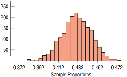
Example: If we repeatedly sample M&Ms and record the proportion of blue candies, the histogram of these proportions forms the sampling distribution.

Properties of the Sampling Distribution for Proportions

Under certain conditions, the sampling distribution of sample proportions is approximately Normal, symmetric, and unimodal. This allows us to use the Normal model to make probability statements and construct confidence intervals.

• Mean: The mean of the sampling distribution is the population proportion \( p \).

• Standard Deviation: The standard deviation is given by:

$\sigma_{\hat{p}} = \sqrt{\frac{pq}{n}}$ where \( p \) is the population proportion, \( q = 1 - p \), and \( n \) is the sample size.

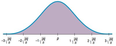
• Normal Model: The sampling distribution of \( \hat{p} \) is approximately Normal:

$\hat{p} \sim N\left(p, \frac{p(1-p)}{n}\right)$

We can use the 68–95–99.7 Rule (empirical rule) or statistical software to calculate probabilities and confidence intervals for proportions.

Sample Distribution vs. Sampling Distribution

It is important to distinguish between the distribution of a sample and the sampling distribution:

• Sample Distribution: The display of data collected in a single sample; no summary statistic has been calculated yet.

• Sampling Distribution: The distribution of summary statistics (e.g., sample proportion) from many different samples.

Key Point: Sampling distributions arise because samples vary, and each random sample will contain different cases and thus a different value of the statistic.

Quantifying Uncertainty and Making Inferences

By studying the sampling distribution, we can quantify the uncertainty in our estimates and make statements about the population parameter. The standard deviation of the sampling distribution (sampling error) tells us how precise our estimates are likely to be.

• Estimating: Guessing the true proportion in the population based on the sample.

• Testing: Assessing how good our guess is by quantifying uncertainty.

• Predicting: Using the sampling distribution to predict the range of likely sample statistics.

Example: If the true proportion of blue M&Ms is 0.24, and we take samples of size 100, the sampling distribution of \( \hat{p} \) will be centered at 0.24 with a standard deviation of $\sqrt{\frac{0.24 \times 0.76}{100}}$.