Sampling Distribution Models and Confidence Intervals for Proportions

Sampling Distribution Models and Confidence Intervals for Proportions

Introduction to Statistical Inference and Sampling

Statistical inference is the process of using data from a sample to make estimates or test hypotheses about a population. The foundation of inference is understanding how sample statistics vary from sample to sample, which is described by the concept of a sampling distribution.

Population, Sample, and Statistical Inference

• Population: The entire group of individuals or items that we want to learn about.

• Sample: A subset of the population, selected to represent the group.

• Statistical Inference: Drawing conclusions about the population based on sample data, using probability models to quantify uncertainty.

The basic cycle of statistics involves collecting data from a sample, analyzing it, and making inferences about the population.

Sampling Variability and Sampling Error

When we draw random samples from a population, the sample statistics (such as the sample proportion) will vary from one sample to another. This variation is called sampling variability or sampling error. Quantifying this uncertainty is essential for making reliable inferences.

• Sampling Variability: The natural variation in statistics from sample to sample.

• Sampling Error: The difference between a sample statistic and the true population parameter.

Sampling Distribution of a Statistic

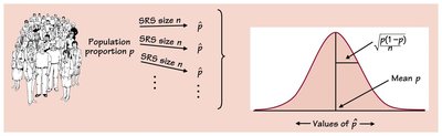
The sampling distribution of a statistic is the probability distribution of that statistic, considered over all possible random samples of a fixed size from the population. For example, the sampling distribution of the sample proportion describes how the sample proportion varies across all possible samples.

• The sampling distribution allows us to make statements about the likely values of the population parameter and the precision of our estimates.

• The standard deviation of the sampling distribution is a measure of sampling variability.

Sampling Distribution Model for a Proportion

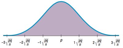
Under certain conditions, the sampling distribution of the sample proportion (\( \hat{p} \)) is approximately Normal (bell-shaped, symmetric, and unimodal). This allows us to use the Normal model to make probability statements about sample proportions.

• Mean of the sampling distribution: \( \mu_{\hat{p}} = p \), where p is the true population proportion.

• Standard deviation (standard error): \( \sigma_{\hat{p}} = \sqrt{\frac{pq}{n}} \), where q = 1 - p and n is the sample size.

As the sample size increases, the sampling distribution becomes more tightly clustered around the true proportion.

Normal Model for Sample Proportions

When the sample size is large enough and the population is not too skewed, the sampling distribution of \( \hat{p} \) can be approximated by a Normal distribution:

• \( \hat{p} \sim N \left( p, \sqrt{\frac{p(1-p)}{n}} \right) \)

• This allows us to use the 68–95–99.7 Rule (empirical rule) or statistical software to calculate probabilities and confidence intervals.

Sample Distribution vs. Sampling Distribution

• Sample Distribution: The distribution of observed data values in a single sample. It is a display of the data collected, not a summary statistic.

• Sampling Distribution: The distribution of a summary statistic (such as the sample proportion) over many random samples. It arises because each sample yields a different value of the statistic.

Understanding the difference is crucial for interpreting statistical results and making valid inferences.

Key Formulas

• Mean of sampling distribution: $\mu_{\hat{p}} = p$

• Standard deviation (standard error): $\sigma_{\hat{p}} = \sqrt{\frac{pq}{n}}$

• Normal approximation: $\hat{p} \sim N \left( p, \sqrt{\frac{p(1-p)}{n}} \right)$

Example Application

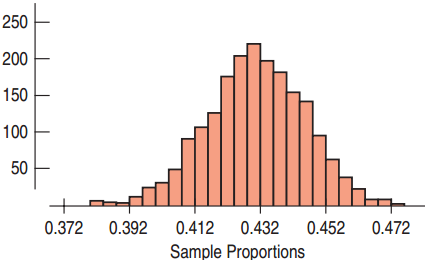
Suppose we want to estimate the proportion of blue M&M's in a large bag. We take several random samples of size n and calculate the sample proportion of blue M&M's in each sample. The distribution of these sample proportions forms the sampling distribution, which is approximately Normal if the sample size is large enough.

Additional info: The images of M&M's and the histogram of sample proportions reinforce the concept of sampling distributions by providing a tangible example and visualizing the variability in sample statistics.