Sampling Distributions and Confidence Intervals: The Central Limit Theorem and Estimation

Sampling Distributions

The Concept of a Sampling Distribution

The sampling distribution of a sample statistic is the probability distribution of that statistic, calculated from all possible samples of a fixed size drawn from a population. The most common statistic considered is the sample mean (\( \bar{x} \)).

• Population parameters: Mean = \( \mu \), Standard deviation = \( \sigma \)

• Sampling distribution of the mean: If we repeatedly draw samples of size n and calculate their means, the distribution of these means forms the sampling distribution.

• Central Limit Theorem (CLT): For large n, the sampling distribution of \( \bar{x} \) is approximately normal, regardless of the population's shape.

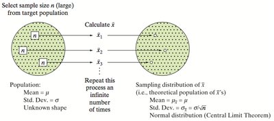
Central Limit Theorem (CLT)

The Central Limit Theorem states that, for a sufficiently large sample size n, the sampling distribution of the sample mean \( \bar{x} \) will be approximately normal, even if the population distribution is not normal. The mean of the sampling distribution is \( \mu_{\bar{x}} = \mu \) and the standard deviation (standard error) is \( \sigma_{\bar{x}} = \frac{\sigma}{\sqrt{n}} \).

• As sample size increases, the sampling distribution becomes more normal and less spread out.

• Standard error (SE): $SE = \frac{\sigma}{\sqrt{n}}$

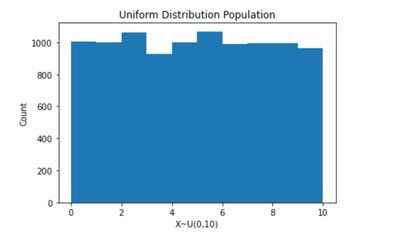
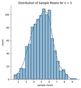
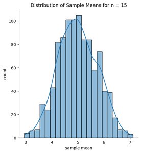
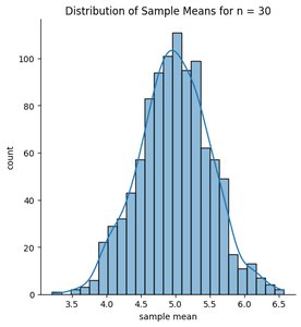
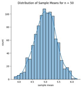
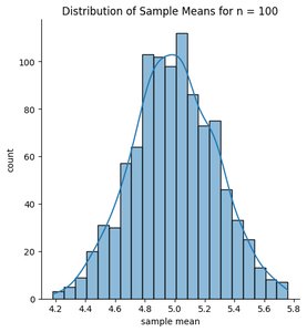
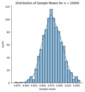
Key Point: The larger the sample size, the better the normal approximation to the sampling distribution of \( \bar{x} \).

Example: Probability Calculation for Sample Mean

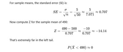
Suppose the population mean is 500, standard deviation is 5, and sample size is 50. What is the probability that the sample mean is less than 490?

• Standard error: $SE = \frac{5}{\sqrt{50}} \approx 0.707$

• Z-score: $Z = \frac{490 - 500}{0.707} \approx -14.14$

• This is extremely far in the left tail, so $P(\bar{X} < 490) \approx 0$

Confidence Intervals for the Population Mean

Concept of Confidence Interval

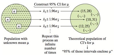
A confidence interval (CI) provides a range of plausible values for a population parameter, such as the mean. It is constructed so that, with a specified probability (confidence level), the interval will contain the true parameter value.

• General formula: $\text{Point Estimate} \pm (\text{Critical Value}) \times (\text{Standard Error})$

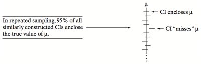
• Interpretation: For a 95% CI, if we repeated the sampling process many times, about 95% of the constructed intervals would contain the true mean \( \mu \).

Critical Values and Confidence Levels

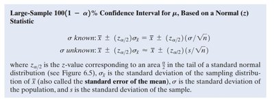
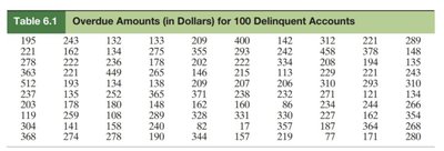
The critical value depends on the desired confidence level and the sampling distribution (z for normal, t for small samples with unknown σ). Commonly used z-values are:

Confidence Level	α	α/2	zα/2
90%	0.10	0.05	1.645
95%	0.05	0.025	1.960
98%	0.02	0.01	2.326
99%	0.01	0.005	2.576

Conditions for Valid Confidence Intervals

• A random sample is selected from the target population.

• Sample size is large (n ≥ 30), so the sampling distribution of \( \bar{x} \) is approximately normal (by CLT).

Formulas for Confidence Intervals

• Large-sample CI for mean (σ known): $\bar{x} \pm z_{\alpha/2} \left( \frac{\sigma}{\sqrt{n}} \right)$

• Large-sample CI for mean (σ unknown): $\bar{x} \pm z_{\alpha/2} \left( \frac{s}{\sqrt{n}} \right)$

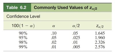
Example: Confidence Interval for Delinquent Accounts

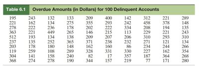
Suppose we have a sample of 100 delinquent accounts with mean $233.28 and standard deviation $90.34. Construct a 95% confidence interval for the population mean.

• Sample mean: $233.28

• Sample standard deviation: $90.34

• Sample size: 100

• Critical value for 95%: 1.96

• Standard error: $\frac{90.34}{\sqrt{100}} = 9.034$

• Margin of error: $1.96 \times 9.034 = 17.71$

• Confidence interval: $233.28 \pm 17.71 = (215.57, 250.99)$

Interpretation: We are 95% confident that the true mean amount owed by all delinquent accounts is between $215.57 and $250.99.

Small-Sample Confidence Intervals (t-distribution)

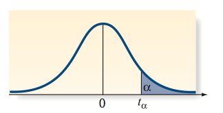
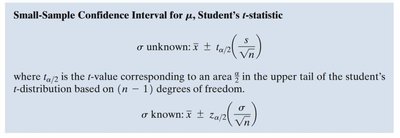
When the population standard deviation is unknown and the sample size is small (n < 30), use the t-distribution:

• Formula: $\bar{x} \pm t_{\alpha/2,\,df} \left( \frac{s}{\sqrt{n}} \right)$

• Degrees of freedom: $df = n - 1$

Summary Table: Commonly Used z Critical Values

Confidence Level	α	α/2	zα/2
90%	0.10	0.05	1.645
95%	0.05	0.025	1.960
98%	0.02	0.01	2.326
99%	0.01	0.005	2.576

Key Takeaways

• The sampling distribution of the mean becomes approximately normal as sample size increases (Central Limit Theorem).

• Confidence intervals provide a range of plausible values for the population mean, with a specified level of confidence.

• For large samples, use the normal (z) distribution; for small samples with unknown σ, use the t-distribution.