Sampling Distributions and the Central Limit Theorem: Study Guide

Sampling Distributions

Definition and Concept

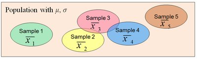
The concept of sampling distributions is fundamental in statistics. A sampling distribution is the probability distribution of a sample statistic (such as the mean or standard deviation) formed when samples of size n are repeatedly taken from a population.

• Population: The entire group of interest, characterized by a mean (μ) and standard deviation (σ).

• Sample: A subset of the population, from which a sample statistic (e.g., sample mean \bar{x}) is calculated.

• Sampling Distribution: The distribution of sample means (or other statistics) from all possible samples of size n.

Example: If you repeatedly draw samples of size n from a population and calculate the mean for each sample, the collection of these means forms the sampling distribution of the sample mean.

Properties of Sampling Distributions of Sample Means

Sampling distributions of sample means have important properties:

• Mean of Sample Means: The mean of the sampling distribution of sample means (\mu_{\bar{x}}) is equal to the population mean (μ).

• Standard Error: The standard deviation of the sampling distribution (\sigma_{\bar{x}}), also called the standard error, is given by:

$\sigma_{\bar{x}} = \frac{\sigma}{\sqrt{n}}$

• Variance of Sample Means: The variance is:

$\sigma^2_{\bar{x}} = \frac{\sigma^2}{n}$

The Central Limit Theorem (CLT)

Statement and Importance

The Central Limit Theorem (CLT) is a cornerstone of inferential statistics. It describes the relationship between the sampling distribution of sample means and the population from which samples are drawn.

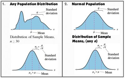
• The CLT states that the sampling distribution of any statistic will be normal or nearly normal if the sample size is large enough (typically n ≥ 30).

• If the population is normally distributed, the sampling distribution of sample means is normal for any sample size n.

• The mean of the sampling distribution is equal to the population mean (\mu_{\bar{x}} = \mu).

• The standard deviation (standard error) is \sigma_{\bar{x}} = \frac{\sigma}{\sqrt{n}}.

Visual Representation

The CLT can be visualized as follows:

• For any population distribution, as sample size increases, the distribution of sample means approaches normality.

• For a normal population, the distribution of sample means is always normal, regardless of sample size.

Applying the Central Limit Theorem

Calculating Mean and Standard Error

To apply the CLT, use the following formulas:

• Mean of Sample Means: $\mu_{\bar{x}} = \mu$

• Standard Error: $\sigma_{\bar{x}} = \frac{\sigma}{\sqrt{n}}$

Example: If the population mean number of eggs laid by house flies is 800 and the standard deviation is 100, for samples of size 15:

• $\mu_{\bar{x}} = 800$

• $\sigma_{\bar{x}} = \frac{100}{\sqrt{15}} \approx 25.82$

Finding Probabilities Using the CLT

To find the probability that a sample mean falls below or above a certain value, convert the sample mean to a z-score:

$z = \frac{\bar{x} - \mu}{\sigma / \sqrt{n}}$

• Use z-tables to find the probability corresponding to the calculated z-score.

Example: If the average weight of 6th graders is 80 pounds (σ = 20), and a sample of 50 students is drawn, what is the probability that the sample mean is less than 75 pounds?

• $\mu_{\bar{x}} = 80$

• $\sigma_{\bar{x}} = \frac{20}{\sqrt{50}}$

• $z = \frac{75 - 80}{20 / \sqrt{50}} \approx -1.77$

• Probability: $P(z < -1.77) = 0.0384$

Examples and Interpretation

Sample Size and Standard Error

As sample size increases, the standard error decreases, making the sampling distribution more concentrated around the population mean.

• Example: For μ = 125, σ = 19:

• n = 39: $\sigma_{\bar{x}} = \frac{19}{\sqrt{39}} \approx 3.04$

• n = 199: $\sigma_{\bar{x}} = \frac{19}{\sqrt{199}} \approx 1.35$

• The mean remains unchanged, but the standard error decreases as n increases.

Probability Calculations

For normally distributed populations, probabilities for sample means can be calculated using the z-score formula and standard normal tables.

• Example: For ice cream cartons (μ = 10, σ = 0.5, n = 35), probability that mean weight is less than 9.81 ounces:

• $z = \frac{9.81 - 10}{0.5 / \sqrt{35}} \approx -2.25$

• Probability: $P(z < -2.25) = 0.0122$

Interpreting Unusual Results

If a calculated probability is less than or equal to 0.05, the result is considered unusual.

• Example: For carbon dioxide emissions, if the probability is 0.0678, it is not considered unusual.

Summary Table: Key Formulas

Statistic	Formula	Description
Mean of Sample Means	$\mu_{\bar{x}} = \mu$	Population mean
Standard Error	$\sigma_{\bar{x}} = \frac{\sigma}{\sqrt{n}}$	Standard deviation of sample means
Variance of Sample Means	$\sigma^2_{\bar{x}} = \frac{\sigma^2}{n}$	Variance of sample means
Z-score for Sample Mean	$z = \frac{\bar{x} - \mu}{\sigma / \sqrt{n}}$	Standardized value