Sampling Distributions and the Central Limit Theorem: Study Notes for Introductory Statistics

Sampling Distributions

Introduction to Sampling Distributions

Sampling distributions are fundamental in statistics for understanding how sample statistics relate to population parameters. When we use a sample statistic to estimate a population parameter, the sampling distribution describes the variability of that statistic across all possible samples of a given size from the population.

• Sample Statistic: A numerical summary (e.g., mean, proportion) calculated from a sample.

• Population Parameter: A numerical summary (e.g., mean, proportion) describing the entire population.

• Sampling distributions allow us to quantify how much a sample statistic is expected to vary from sample to sample.

Sampling Distribution of a Proportion

The sampling distribution of a sample proportion describes the distribution of proportions calculated from all possible samples of a fixed size from a population.

• Sample Proportion (\( \hat{p} \)): The proportion of successes in a sample, defined as \( \hat{p} = \frac{X}{n} \), where X is the number of successes and n is the sample size.

• The sample proportion varies from sample to sample, and the distribution of these proportions is called the sampling distribution of the sample proportion.

Properties of the Sampling Distribution for a Proportion

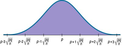
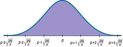
• Expected Value: \( \mu_{\hat{p}} = p \), where p is the true population proportion.

• Standard Deviation: \( SD_{\hat{p}} = \sqrt{\frac{p q}{n}} \), where q = 1 - p.

• Shape: For large enough sample sizes, the sampling distribution of \( \hat{p} \) is approximately Normal (by the Central Limit Theorem).

Example: Estimating Proportion of Premature Births

• Population parameter: 11.6% of U.S. live births in 1998 were premature (\( p = 0.116 \)).

• For samples of size \( n = 100 \):

  • \( \mu_{\hat{p}} = 0.116 \)

  • \( SD_{\hat{p}} = \sqrt{\frac{0.116 \times 0.884}{100}} = 0.032 \)

Simulation Example: Free Throw Shooting

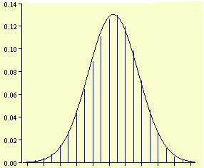
Simulations can illustrate how sample proportions vary. For example, simulating 50 free throws for a 75% shooter shows the variability in the number of successful shots across samples.

• Expected number of made free throws: \( 0.75 \times 50 = 37.5 \)

• Standard deviation: \( SD_{\hat{p}} = \sqrt{\frac{0.75 \times 0.25}{50}} = 0.06124 \)

Assumptions and Conditions for Normality

To use the Normal model for the sampling distribution of proportions, certain assumptions and conditions must be met:

• Independence Assumption: Data values must be independent.

• Randomization Condition: The sample should be a simple random sample.

• 10% Condition: The sample size should be no more than 10% of the population.

• Success/Failure Condition: Both \( np \geq 10 \) and \( nq \geq 10 \).

Example: U.S. Live Births in 1998

• Sample: 925 births, 124 premature (\( \hat{p} = \frac{124}{925} = 0.134 \)).

• Check conditions: Randomization, 10%, Success/Failure all satisfied.

• Standard deviation: \( SD_{\hat{p}} = 0.011 \)

• 95% of sample proportions should fall within \( 0.116 \pm 2 \times 0.011 = [0.094, 0.138] \).

• Observed \( \hat{p} = 0.134 \) is within this range; z-score is \( z = \frac{0.134 - 0.116}{0.011} = 1.71 \).

The Central Limit Theorem (CLT)

Introduction to the Central Limit Theorem

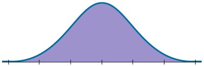
The Central Limit Theorem (CLT) is a foundational result in statistics. It states that the sampling distribution of the sample mean (or proportion) becomes approximately Normal as the sample size increases, regardless of the population's distribution, provided the sample size is large enough.

• For Means: The distribution of sample means is approximately Normal for large n.

• For Proportions: The distribution of sample proportions is approximately Normal for large n.

Assumptions and Conditions for Means

• Independence Assumption: Data values must be independent.

• Randomization Condition: The sample should be a simple random sample.

• 10% Condition: The sample size should be no more than 10% of the population.

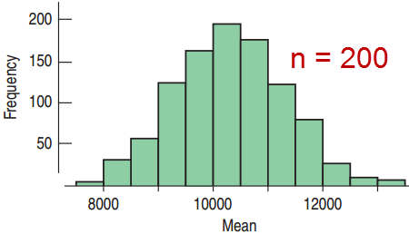
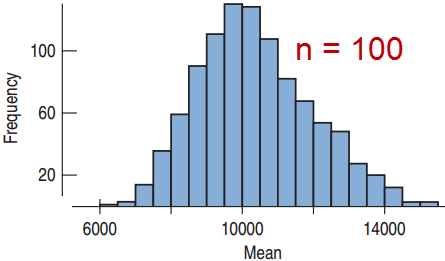
• Large Enough Condition: For unimodal and symmetric populations, \( n \geq 25 \) is usually sufficient; for skewed populations, \( n \geq 100 \) may be needed.

Shape of the Sampling Distribution for Means

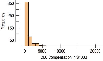
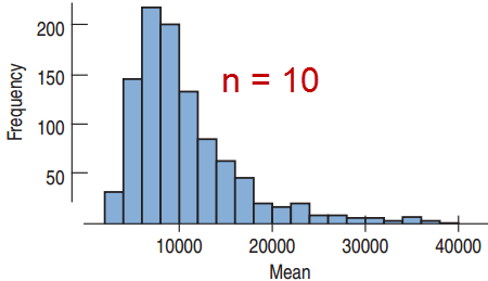
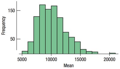
• The more non-normal the population, the larger the sample size needed for the sampling distribution of the mean to be approximately Normal.

• The Law of Large Numbers states that as n increases, the sample mean approaches the population mean.

Parameters of the Normal Model for Sampling Distributions

• For Proportions: Centered at \( p \), standard deviation \( \sqrt{\frac{p q}{n}} \).

• For Means: Centered at \( \mu \), standard deviation \( \frac{\sigma}{\sqrt{n}} \), where \( \sigma \) is the population standard deviation.

Application Example: Balcony Capacity

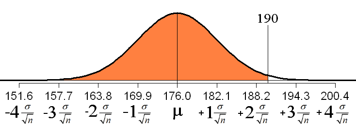
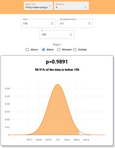
Suppose an architect wants to ensure a balcony can safely support 100 adults. The mean adult weight is 176 lbs (\( \mu = 176 \)), with a standard deviation of 61 lbs (\( \sigma = 61 \)). The balcony is designed for 19,000 lbs.

• We want \( P(\text{total weight} < 19,000) \), or equivalently, \( P(\bar{y} < 190) \).

• Check conditions: Randomization, 10%, Large Enough (\( n = 100 \)).

• \( \mu_{\bar{y}} = 176 \), \( SD_{\bar{y}} = \frac{61}{\sqrt{100}} = 6.1 \)

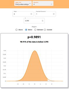
• \( z = \frac{190 - 176}{6.1} = 2.295 \)

• Probability: About 98.9% chance the average weight is below 190 lbs; 1.1% chance it exceeds capacity.

Summary Table: Key Formulas for Sampling Distributions

Statistic	Expected Value (Mean)	Standard Deviation	Shape (for large n)
Sample Proportion (\( \hat{p} \))	\( p \)	\( \sqrt{\frac{p q}{n}} \)	Approximately Normal
Sample Mean (\( \bar{y} \))	\( \mu \)	\( \frac{\sigma}{\sqrt{n}} \)	Approximately Normal

Why Are Sampling Distributions Important?

• They allow us to make inferences about population parameters using sample data.

• They quantify the typical difference between a sample statistic and the population parameter (sampling variability).

• They are the foundation for constructing confidence intervals and conducting hypothesis tests.