Sampling Distributions and the Sample Mean

Sampling Distributions

Introduction to Sampling Distributions

Sampling distributions describe the behavior of sample statistics, such as the sample mean or sample proportion, when many random samples are drawn from a population. Understanding these distributions is crucial for making statistical inferences about populations based on sample data.

• Statistic: A numerical value calculated from sample data (e.g., sample mean Y̅, sample standard deviation S).

• Parameter: A numerical value that describes the entire population (e.g., population mean μ, population standard deviation σ).

Examples

• Quantitative Variable:

  • Sample Mean: Y̅

  • Population Mean: μ

  • Sample Standard Deviation: S

  • Population Standard Deviation: σ

• Categorical Variable:

  • Population Proportion: p (true proportion in the population)

  • Sample Proportion: ̂p ("p-hat")

Formula for Sample Proportion:

$\hat{p} = \frac{\text{Count}}{n}$

Sampling Distribution of the Sample Mean (Y̅)

Understanding the Sampling Distribution

The sampling distribution of the sample mean is the probability distribution of all possible values of the sample mean (Y̅) that could be obtained from repeated random samples of a fixed size from a population.

• Different samples produce different values for Y̅.

• The sample means (Y̅'s) tend to be close to the population mean (μ).

• The sample means have less variability than individual values from the population.

Example: Word Lengths in the Gettysburg Address

• Population: All words in the Gettysburg Address

• Variable: Length of a word (in letters)

• Population Mean (μ): 4.3 letters

• Population Standard Deviation (σ): 2.1 letters

• Distribution Shape: Skewed to the right

• Range: Minimum 1 letter, Maximum 11 letters, Median 4 letters

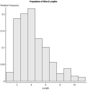
Figure: Histogram showing the distribution of word lengths in the population. The distribution is right-skewed, with most words having 2-5 letters.

Sampling Distribution Properties

• The sampling distribution of Y̅ is centered around the population mean (μ).

• It has less variability than the population distribution.

• For large sample sizes, the sampling distribution becomes approximately normal, regardless of the population's shape (Central Limit Theorem).

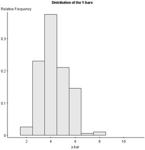
Figure: Histogram showing the distribution of sample means (Y̅) from many samples. The distribution is less skewed and more concentrated around the mean compared to the population distribution.

Theoretical Properties of the Sampling Distribution of Y̅

• Mean: $\mu_{\overline{Y}} = \mu$

• Standard Deviation (Standard Error): $SD(\overline{Y}) = \frac{\sigma}{\sqrt{n}}$

• Shape: For large samples (n ≥ 30), the sampling distribution is approximately normal (Central Limit Theorem). For smaller samples, the population should be nearly normal for this approximation to hold.

Central Limit Theorem (CLT)

The Central Limit Theorem states that, for sufficiently large sample sizes, the sampling distribution of the sample mean will be approximately normal, regardless of the population's distribution.

• "Large" sample size: Typically, n ≥ 30 is considered sufficient.

• For smaller samples, the population distribution should be nearly normal.

Standardizing the Sample Mean

To answer probability questions about the sample mean, we can standardize Y̅ using the following formula:

$Z = \frac{\overline{Y} - \mu_{\overline{Y}}}{SD(\overline{Y})}$

This allows us to use the standard normal distribution to find probabilities related to the sample mean.

Example Application

• Suppose we take many samples of size 5 from the population of word lengths in the Gettysburg Address and calculate their means. The distribution of these means will be centered at 4.3 letters, with less variability than the original population, and will be less skewed.

Additional info: The Central Limit Theorem is foundational for inferential statistics, as it justifies the use of normal probability models for sample means, even when the population is not normal, provided the sample size is large enough.