Sampling Distributions, Central Limit Theorem, and Confidence Intervals

Sampling Distributions and the Central Limit Theorem

Sampling Distribution for the Sample Mean

The sampling distribution of the sample mean is the probability distribution of all possible sample means of a given size from a population. This concept is fundamental in inferential statistics, as it allows us to estimate population parameters using sample statistics.

• Sample Mean (\(\overline{X}\)): The average value from a sample, used to estimate the population mean (\(\mu\)).

• When multiple samples of the same size are taken, the distribution of their means forms the sampling distribution of \(\overline{X}\).

• The mean of the sampling distribution of \(\overline{X}\) is equal to the population mean \(\mu\).

• The standard deviation of the sampling distribution (standard error) is \(\sigma_{\overline{X}} = \frac{\sigma}{\sqrt{n}}\), where \(\sigma\) is the population standard deviation and \(n\) is the sample size.

• As the sample size increases, the sampling distribution becomes more concentrated around the population mean.

Example: A pet store estimates the average number of pets owned by households by taking several samples of 30 Americans. The average of the sample means provides a better approximation of the population mean than a single sample mean.

The Central Limit Theorem (CLT)

The Central Limit Theorem states that for any random variable \(X\), as the sample size \(n\) increases, the sampling distribution of the sample mean \(\overline{X}\) approaches a normal distribution, regardless of the shape of the population distribution.

• For large \(n\), \(\overline{X}\) is approximately normal, even if the population distribution is not normal.

• Rule of thumb: \(n \geq 30\) is often considered sufficient for the CLT to apply.

• This allows us to use z-scores and normal probability tables to calculate probabilities for sample means.

Formula for z-score of a sample mean:

$z = \frac{\overline{x} - \mu}{\sigma / \sqrt{n}}$

Example: If the mean play time for a game is 26.7 hours based on 100 samples of 40 players, then \(n = 40\).

Confidence Intervals for Population Mean

Introduction to Confidence Intervals

A confidence interval (CI) is a range of values, derived from sample statistics, that is likely to contain the value of an unknown population parameter. The confidence level (e.g., 95%) indicates the probability that the interval contains the parameter.

• Point Estimate: A single value estimate of a parameter (e.g., sample mean).

• Confidence Interval: An interval estimate, typically written as (lower bound, upper bound) or \(\hat{y} \pm E\), where \(E\) is the margin of error.

• Margin of Error (E): The maximum expected difference between the point estimate and the true parameter value.

• Confidence Level (C): The probability that the CI contains the parameter, denoted as \(1-\alpha\).

Formula for Confidence Interval (when \(\sigma\) known):

$\overline{x} \pm z_{\alpha/2} \cdot \frac{\sigma}{\sqrt{n}}$

Formula for Confidence Interval (when \(\sigma\) unknown):

$\overline{x} \pm t_{\alpha/2} \cdot \frac{s}{\sqrt{n}}$

Example: If a sample mean is 4 and the margin of error is 2, the 95% CI is (2, 6).

Critical Values: z and t Distributions

Critical values are used to determine the margin of error for confidence intervals.

• z-distribution: Used when the population standard deviation \(\sigma\) is known and the sample size is large (\(n \geq 30\)).

• t-distribution: Used when \(\sigma\) is unknown and the sample size is small (\(n < 30\)). The t-distribution is wider and depends on degrees of freedom (df = n - 1).

Common z critical values:

Confidence Level	z\(\alpha/2\)
90%	1.645
95%	1.960
99%	2.576

t critical values are found using a t-table or calculator, based on confidence level and degrees of freedom.

Constructing Confidence Intervals: Step-by-Step

1. Verify sample is random and population is normal or \(n > 30\).

2. Find the appropriate critical value (z or t).

3. Calculate the margin of error.

4. Compute the lower and upper bounds of the interval.

Example: For a sample mean of $3.50, \(\sigma = 0.04\), \(n = 100\), and 80% confidence, use the formula above to construct the CI.

Using Technology (TI-84) for Confidence Intervals

Most calculators have built-in functions for constructing confidence intervals:

• For mean: ZInterval (if \(\sigma\) known), TInterval (if \(\sigma\) unknown)

• For proportion: 1-PropZInterval

Determining Minimum Sample Size

Sample Size for Mean

To achieve a desired margin of error, the minimum sample size \(n\) can be calculated by rearranging the margin of error formula:

$n = \left( \frac{z_{\alpha/2} \cdot \sigma}{E} \right)^2$

If \(\sigma\) is unknown, estimate using the range rule of thumb: $s \approx \frac{\text{range}}{4}$

Sample Size for Proportion

For proportions, the minimum sample size is:

$n = \frac{z_{\alpha/2}^2 \cdot p(1-p)}{E^2}$

If \(p\) is unknown, use \(p = 0.5\) for the most conservative estimate.

Confidence Intervals for Population Proportion

Constructing Confidence Intervals for Proportions

For a population proportion \(p\), the confidence interval is constructed as follows:

• Point estimate: \(\hat{p} = \frac{x}{n}\), where \(x\) is the number of successes in the sample.

• Margin of error: $E = z_{\alpha/2} \cdot \sqrt{\frac{\hat{p}(1-\hat{p})}{n}}$

• Confidence interval: $\hat{p} \pm E$

• Conditions: Both \(np \geq 5\) and \(n(1-p) \geq 5\) for normal approximation.

Example: In a sample of 200 people, 90 prefer Brand A. The 90% CI for the proportion is calculated using the formulas above.

Confidence Intervals for Variance and Standard Deviation

Chi-Square Distribution

The chi-square (\(\chi^2\)) distribution is used to construct confidence intervals for population variance and standard deviation. It is not symmetric and always positive.

• Degrees of freedom: \(df = n - 1\)

• Critical values: \(\chi^2_{\alpha/2}\) (right tail) and \(\chi^2_{1-\alpha/2}\) (left tail) are found using a chi-square table.

Confidence interval for variance (\(\sigma^2\)):

$\left( \frac{(n-1)s^2}{\chi^2_{\alpha/2}}, \frac{(n-1)s^2}{\chi^2_{1-\alpha/2}} \right)$

For standard deviation, take the square root of the interval endpoints.

Example: For a sample variance of 1.2 (n = 12), construct a 90% CI for the population variance using the chi-square distribution.

Using the Normal Distribution to Approximate Binomial Probabilities

Normal Approximation to the Binomial

When the number of trials \(n\) is large and both \(np\) and \(n(1-p)\) are at least 5, the binomial distribution can be approximated by the normal distribution. A continuity correction of 0.5 is applied when using the normal approximation.

• Mean: \(\mu = np\)

• Standard deviation: \(\sigma = \sqrt{np(1-p)}\)

• z-score: $z = \frac{x - \mu}{\sigma}$

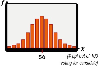
Example: If 56 out of 100 people vote for a candidate with probability 0.56, use the normal approximation to find probabilities for more than 60 votes.

Summary Table: Critical Values for t-Distribution (Selected df)

df	80%	90%	95%	98%	99%
1	3.078	6.314	12.706	31.821	63.657
5	1.476	2.015	2.571	3.365	4.032
10	1.372	1.812	2.228	2.764	3.169
30	1.310	1.697	2.042	2.457	2.750
∞	1.282	1.645	1.960	2.326	2.576

Additional info: For more detailed tables, refer to the t-distribution and chi-square tables in your textbook or statistical appendix.