Sampling Distributions for Proportions and Means: Key Concepts and Applications

Sampling Distributions

Population vs. Sample

In statistics, a population refers to the entire group of individuals or items of interest, while a sample is a subset of the population selected for study. Inferential statistics use information from samples to make conclusions about populations.

• Population: The complete set of individuals, items, or data.

• Sample: A smaller group drawn from the population, used to estimate population characteristics.

Parameter vs. Statistic

A parameter is a numerical value summarizing a characteristic of the population (e.g., mean, proportion), while a statistic is a numerical value summarizing a characteristic of the sample.

• Parameter: Constant value calculated from the entire population.

• Statistic: Value calculated from the sample, used to estimate the parameter.

Example: If the average height of all students in a class is 65 inches (parameter), and the average height in a sample of 10 students is 64 inches (statistic), the sample statistic estimates the population parameter.

Sampling Distributions of the Sample Mean (x̄)

Definition and Properties

The sampling distribution of the sample mean (x̄) is the distribution of all possible sample means from samples of a given size (n) drawn from the population.

• Shape: The shape of the sampling distribution depends on the population distribution and sample size.

• Center: The mean of the sampling distribution equals the population mean (μ).

• Spread: The spread is measured by the standard error of the mean.

Standard Error of the Mean

The standard error quantifies the variability of sample means around the population mean. It is calculated as:

$\sigma_{\bar{x}} = \frac{\sigma}{\sqrt{n}}$

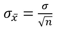
Example: If the population standard deviation is 10 and the sample size is 25, the standard error is $\frac{10}{\sqrt{25}} = 2$.

Central Limit Theorem (CLT)

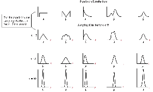
The Central Limit Theorem states that, for sufficiently large sample sizes, the sampling distribution of the sample mean (x̄) will be approximately normal, regardless of the population's distribution.

• Normality: The distribution of x̄ approaches normal as n increases.

• Mean: $\mu_{\bar{x}} = \mu$

• Standard Error: $\sigma_{\bar{x}} = \frac{\sigma}{\sqrt{n}}$

Assumptions:

• Random sample

• Independence

• Sample size: n ≥ 30 for skewed distributions; n ≥ 10-20 for slightly skewed; n ≥ 5-10 for normal distributions

Applications and Examples

• WIC Program Example: Population of 9407 mothers, mean month of prenatal care initiation is 2.649, SD is 1.975.

• Anthropologist Example: Population mean family size is 5.2, SD is 2.0, sample mean is 4.6, sample SD is 3.2 for n=36.

• GMAT Example: Population mean is 500, SD is 110. For n=100, standard error is $\frac{110}{\sqrt{100}} = 11$.

Sampling Distributions of Sample Proportion (p̂)

Definition and Properties

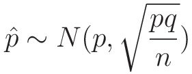
The sample proportion (p̂) is the fraction of items in a sample with a certain characteristic. The sampling distribution of p̂ describes the distribution of sample proportions from repeated samples.

• Mean: $\mu_{\hat{p}} = p$

• Standard Error: $\sigma_{\hat{p}} = \sqrt{\frac{pq}{n}}$ where $q = 1 - p$

Normality Conditions

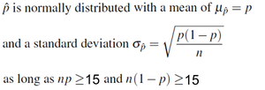
The sampling distribution of p̂ is approximately normal if:

• $n p \geq 15$

• $n (1-p) \geq 15$

Example: California Election Exit Polls

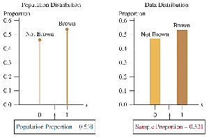
In a poll of 3889 voters, 53.1% voted for Brown. The population proportion was 0.538. The sample proportion closely estimates the population proportion, demonstrating the usefulness of sampling distributions.

Applications and Examples

• Government Data Example: If 6% of the population is at least 75 years old, and n=100, check if $n p = 6$ and $n (1-p) = 94$; since $n p < 15$, normality does not hold.

• Bank Loan Example: If 8% default, n=200, $n p = 16$, $n (1-p) = 184$; normality holds. Mean is 0.08, standard error is $\sqrt{\frac{0.08 \times 0.92}{200}}$.

Summary Table: Sampling Distributions

Type	Mean	Standard Error	Normality Condition
Sample Mean (x̄)	$\mu$	$\frac{\sigma}{\sqrt{n}}$	n ≥ 30 for skewed distributions
Sample Proportion (p̂)	$p$	$\sqrt{\frac{pq}{n}}$	$n p \geq 15$ and $n (1-p) \geq 15$

Key Takeaways

• Sampling distributions allow us to estimate how close sample statistics are to population parameters.

• The Central Limit Theorem is fundamental for understanding the normality of sampling distributions.

• Standard error decreases as sample size increases, improving the precision of estimates.

• Normality conditions must be checked before applying normal probability models to sample means or proportions.