Sampling Distributions of Sample Proportions

Sampling Distributions

Introduction to Sampling Distributions

The concept of a sampling distribution is fundamental in statistics, describing how a statistic (such as a sample proportion) varies from sample to sample. Understanding sampling distributions allows us to make probabilistic statements about how likely it is to observe certain values of a statistic, given a known population parameter.

How Sample Proportions Vary Around the Population Proportion

Population Proportion

• Population proportion (p): The true proportion of individuals in a population with a certain characteristic.

• In practice, the population proportion is often unknown and must be estimated from sample data.

• Example: If we are interested in the proportion of students who live off-campus, p represents the true proportion in the entire student population.

Sample Proportion

• Sample proportion (\( \hat{p} \)): The proportion of individuals with a certain characteristic in a sample, used as an estimate of the population proportion.

• Calculated as: $\hat{p} = \frac{x}{n}$ where x is the number of individuals in the sample with the characteristic, and n is the sample size.

• Example: If 60 out of 100 surveyed students live off-campus, $\hat{p} = \frac{60}{100} = 0.60$.

Sampling Proportion as a Random Variable

• The sample proportion $\hat{p}$ is a random variable because its value changes with different random samples.

• The sampling distribution of $\hat{p}$ describes the distribution of all possible values of $ \hat{p} $ for samples of size n from the population.

Describing the Sampling Distribution of a Sample Proportion

• Shape: As the sample size increases, the sampling distribution of $\hat{p}$ becomes approximately normal (bell-shaped), provided certain conditions are met.

• Center: The mean of the sampling distribution is equal to the population proportion: $\mu_{\hat{p}} = p$

• Variability: The standard deviation (also called the standard error) of the sampling distribution is: $\sigma_{\hat{p}} = \sqrt{ \frac{p(1-p)}{n} }$

• Normal Approximation Conditions: The sampling distribution of $\hat{p}$ is approximately normal if both $np \geq 15$ and $n(1-p) \geq 15$.

Computing Probabilities for Sample Proportions

Using the Normal Approximation

• When the normal approximation conditions are met, probabilities involving $\hat{p}$ can be computed using the standard normal (z) distribution.

• To find the probability that $\hat{p}$ is less than or equal to a certain value, convert $ \hat{p} $ to a z-score:

$z = \frac{ \hat{p} - p }{ \sqrt{ \frac{p(1-p)}{n} } }$

• Use the standard normal table or technology to find the probability corresponding to the calculated z-score.

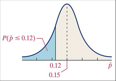
Example: Probability Calculation

• Suppose 15% of all Americans have hearing trouble ($p = 0.15$). In a random sample of 120 Americans ($n = 120$), what is the probability that at most 12% have hearing trouble ($\hat{p} \leq 0.12$)?

• Check normal approximation conditions: $np = 120 \times 0.15 = 18$, $n(1-p) = 120 \times 0.85 = 102$ (both ≥ 15).

• Mean: $\mu_{\hat{p}} = 0.15$

• Standard deviation: $\sigma_{\hat{p}} = \sqrt{ \frac{0.15 \times 0.85}{120} } \approx 0.0325$

• Convert $\hat{p} = 0.12$ to a z-score: $z = \frac{0.12 - 0.15}{0.0325} \approx -0.92$

• Probability: $P(z \leq -0.92) \approx 0.1788$

• Interpretation: There is about a 17.88% chance that at most 12% of a random sample of 120 Americans will have hearing trouble.

Example: Interpreting Unusual Results

• Suppose a sample of 120 Americans who regularly listen to music with headphones yields 26 with hearing trouble ($\hat{p} = \frac{26}{120} \approx 0.217$).

• To determine if this is unusual, compute $P(\hat{p} \geq 0.217)$ under the assumption $p = 0.15$.

• Convert $\hat{p} = 0.217$ to a z-score: $z = \frac{0.217 - 0.15}{0.0325} \approx 2.06$

• Probability: $P(z \leq 2.06) \approx 0.9803$, so $P(\hat{p} \geq 0.217) = 1 - 0.9803 = 0.0197$

• Interpretation: There is about a 1.97% chance of observing a sample proportion of 0.217 or higher if the true population proportion is 0.15. This is considered unusual (less than 5%).

Drawing Conclusions

• If the probability of observing a sample proportion as extreme as the one obtained is very low, we may suspect that the true population proportion is different from the assumed value.

• In the example, it is more plausible that the population proportion of Americans with hearing trouble who regularly listen to music with headphones is higher than 0.15.

Summary Table: Key Quantities for Sampling Distribution of Sample Proportion

Quantity	Symbol	Formula	Description
Population Proportion	p	—	True proportion in the population
Sample Proportion	\( \hat{p} \)	$\hat{p} = \frac{x}{n}$	Proportion in the sample
Mean of Sampling Distribution	$\mu_{\hat{p}}$	$p$	Expected value of $\hat{p}$
Standard Deviation of Sampling Distribution	$\sigma_{\hat{p}}$	$\sqrt{ \frac{p(1-p)}{n} }$	Variability of $\hat{p}$
Normal Approximation Conditions	—	$np \geq 15$ and $n(1-p) \geq 15$	When sampling distribution is approximately normal