Sampling Distributions: Sample Means and Proportions

Study Guide - Smart Notes

Tailored notes based on your materials, expanded with key definitions, examples, and context.

Sampling Distributions

Definition and Importance

The sampling distribution of a statistic is the probability distribution of all possible values of the statistic computed from samples of a fixed size n drawn from a population. This concept is fundamental in inferential statistics, as it allows us to understand the variability of sample statistics and make probabilistic statements about population parameters.

Sample Mean (\( \bar{x} \)): The sampling distribution of the sample mean is the distribution of all possible sample means from samples of size n from a population with mean \( \mu \) and standard deviation \( \sigma \).
Sample Proportion (\( \hat{p} \)): The sampling distribution of the sample proportion is the distribution of all possible sample proportions from samples of size n from a population with proportion p.

Distribution of the Sample Mean

Sample Mean from a Normal Population

When the population is normally distributed, the sampling distribution of the sample mean is also normal, regardless of the sample size. The mean of the sampling distribution equals the population mean, and the standard deviation (standard error) decreases as sample size increases.

Mean of the sampling distribution: \( \mu_{\bar{x}} = \mu \)
Standard deviation (standard error): \( \sigma_{\bar{x}} = \frac{\sigma}{\sqrt{n}} \)

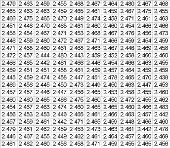
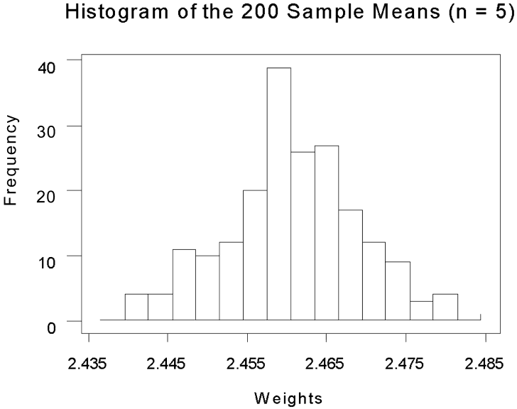
Example: The weights of pennies minted after 1982 are approximately normally distributed with mean 2.46 grams and standard deviation 0.02 grams. If we take 200 simple random samples of size n = 5, the sample means are distributed around the population mean with reduced variability.

Table of 200 sample means for n=5 Histogram of the 200 sample means (n=5)

As the sample size increases (e.g., n = 20), the distribution of the sample means becomes more concentrated around the population mean, and the standard deviation decreases.

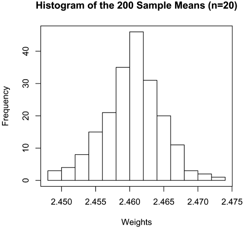
Histogram of the 200 sample means (n=20)

Key Point: Increasing sample size reduces the standard error, making the sample mean a more precise estimator of the population mean.

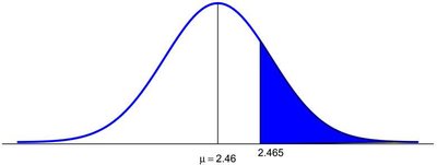
Probability Calculations with the Sample Mean

Probabilities involving the sample mean can be computed using the normal distribution if the population is normal or the sample size is large (Central Limit Theorem). For example, to find the probability that the sample mean exceeds a certain value, convert to a Z-score:

\( Z = \frac{\bar{x} - \mu}{\sigma_{\bar{x}}} \)

Normal curve showing probability area for sample mean

Sample Mean from a Non-Normal Population and the Central Limit Theorem

When the population is not normal, the Central Limit Theorem (CLT) states that the sampling distribution of the sample mean becomes approximately normal as the sample size increases, regardless of the population's shape.

CLT: For sufficiently large n, \( \bar{x} \) is approximately normal with mean \( \mu \) and standard deviation \( \frac{\sigma}{\sqrt{n}} \).

Example: Rolling a fair die (population is not normal):

Distribution of a fair die

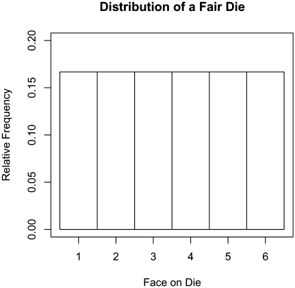
Sampling distributions for different sample sizes:

Histogram of 200 sample means (n=4)

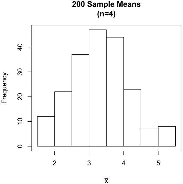
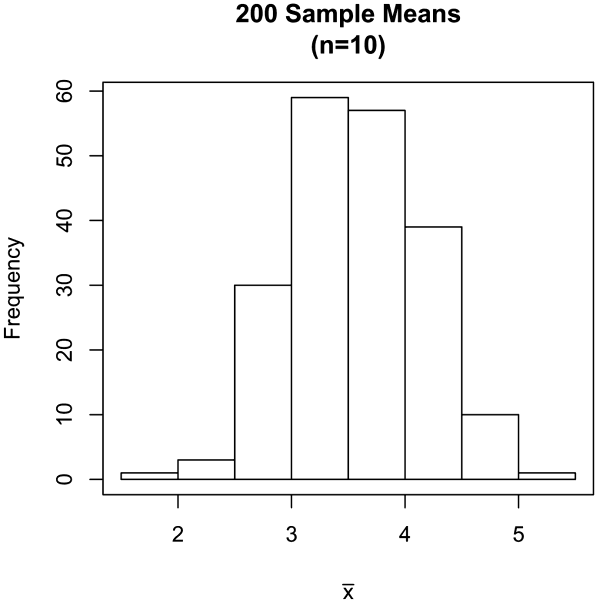
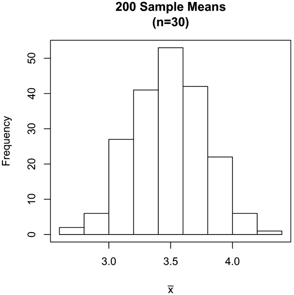
As n increases, the sampling distribution becomes more symmetric and bell-shaped, illustrating the CLT.

Distribution of the Sample Proportion

Sample Proportion: Definition and Properties

The sample proportion \( \hat{p} \) is the fraction of individuals in a sample with a certain characteristic. It is a point estimate of the population proportion p:

\( \hat{p} = \frac{x}{n} \), where x is the number with the characteristic in a sample of size n.

Example: In a poll, 349 out of 1,745 voters approve of a policy. The sample proportion is \( \hat{p} = \frac{349}{1745} = 0.2 \).

Sampling Distribution of the Sample Proportion

The sampling distribution of \( \hat{p} \) describes the variability of sample proportions from repeated samples. For large enough n, the distribution is approximately normal:

Mean: \( \mu_{\hat{p}} = p \)
Standard deviation (standard error): \( \sigma_{\hat{p}} = \sqrt{\frac{p(1-p)}{n}} \)
Normality condition: The distribution is approximately normal if \( np(1-p) \geq 10 \).

Simulated sampling distributions for different sample sizes (n = 10, 50, 100) show that as n increases, the distribution becomes more normal and less spread out:

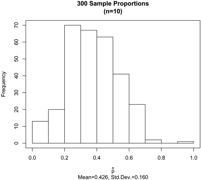
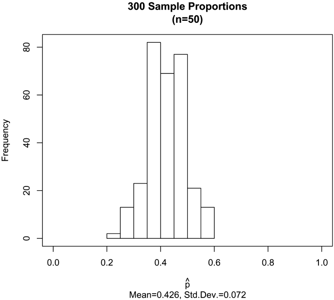
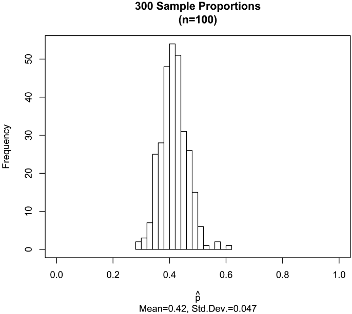
Histogram of 300 sample proportions (n=10)

Key Point: Larger sample sizes yield sampling distributions of \( \hat{p} \) that are more tightly clustered around the population proportion and more closely approximate normality.

Probability Calculations with Sample Proportions

Probabilities involving sample proportions can be computed using the normal approximation when conditions are met. For example, to find the probability that \( \hat{p} \) exceeds a certain value, use:

\( Z = \frac{\hat{p} - p}{\sigma_{\hat{p}}} \)

Interpretation of results should consider whether the observed sample proportion is likely or unusual under the assumed population proportion.

Summary Table: Key Formulas for Sampling Distributions

Statistic	Mean of Sampling Distribution	Standard Deviation (Standard Error)	Approximate Normality Condition
Sample Mean (\( \bar{x} \))	\( \mu_{\bar{x}} = \mu \)	\( \sigma_{\bar{x}} = \frac{\sigma}{\sqrt{n}} \)	Population normal or n large (CLT)
Sample Proportion (\( \hat{p} \))	\( \mu_{\hat{p}} = p \)	\( \sigma_{\hat{p}} = \sqrt{\frac{p(1-p)}{n}} \)	\( np(1-p) \geq 10 \)