STAT 243Z Exam 1 Review: Foundations of Statistics

Ch. 1: Introduction to Statistics

Key Definitions

Statistics is the science of collecting, analyzing, interpreting, and presenting data. Understanding basic terminology is essential for interpreting statistical results.

• Population: The entire group of individuals or items of interest.

• Parameter: A numerical summary describing a characteristic of a population.

• Sample: A subset of the population selected for study.

• Statistic: A numerical summary describing a characteristic of a sample.

• Census: A study that collects data from every member of the population.

Sampling Methods and Bias

• Random Sample: Each member of the population has an equal chance of being selected.

• Simple Random Sample: Every possible sample of a given size has an equal chance of being chosen.

• Bias: Systematic error that skews results; eliminated by randomization and careful sampling.

• Sampling Error: Difference between sample statistic and population parameter due to random chance.

• Nonsampling Error: Errors not related to sampling, such as measurement or data entry mistakes.

• Voluntary Response Sample: Participants self-select; often leads to bias.

• Convenience Sampling: Selecting individuals easiest to reach; may not represent the population.

Types of Data

• Categorical Data: Data that can be grouped by categories (e.g., gender, color).

• Quantitative Data: Numerical data; can be discrete (countable) or continuous (measurable).

• Discrete Data: Countable values (e.g., number of students).

• Continuous Data: Measurable values (e.g., height, weight).

Study Designs

• Experiment: Researcher manipulates variables to observe effects.

• Observational Study: Researcher observes without intervention.

• Practical vs. Statistical Significance: Statistical significance means results are unlikely due to chance; practical significance means results are meaningful in real-world context.

Ch. 2: Exploring Data with Tables and Graphs

Frequency Tables and Histograms

Frequency tables and histograms are foundational tools for summarizing and visualizing quantitative data.

• Class Width: The difference between consecutive lower class limits.

• Class Limits: The smallest and largest values in each class.

• Relative Frequency: The proportion of data values in each class.

• Histogram: A bar graph representing frequency distribution; x-axis should be labeled with class boundaries, not both upper and lower limits.

Other Graphs

• Stem & Leaf Plots: Show individual data values; similar to histograms but preserve original data.

• Dotplots: Display each data point as a dot; useful for small datasets.

• Pie Charts: Represent categorical data; show proportions. Advantages: Easy to interpret proportions. Disadvantages: Not suitable for quantitative data.

• Bar Charts: Used for nominal or ordinal data; bars represent frequency or proportion.

• Time Series Charts: Line graphs showing data trends over time.

Ch. 3: Describing, Exploring, and Comparing Data

Measures of Center

Measures of center describe the typical value in a dataset.

• Mean: Arithmetic average; sensitive to outliers.

• Median: Middle value; resistant to outliers.

• Mode: Most frequent value.

• Midrange: Average of the maximum and minimum values.

• Weighted Mean: Used when values have different weights (e.g., GPA calculation).

• 10% Trimmed Mean: Mean calculated after removing the lowest and highest 10% of values.

Skewed Distribution: In a skewed distribution, mean, median, mode, and midrange differ. Median is most resistant to outliers.

Measures of Variation

Variation measures describe the spread of data values.

• Range: Difference between maximum and minimum values.

• Variance: Average squared deviation from the mean. For a sample: $s^2 = \frac{\sum (x_i - \bar{x})^2}{n-1}$

• Standard Deviation: Square root of variance; measures average distance from the mean. $s = \sqrt{s^2}$

• Symbols: $\sigma$ (population standard deviation), $\mu$ (population mean), $s$ (sample standard deviation), $\bar{x}$ (sample mean)

• Why Standard Deviation? Standard deviation is in the same units as the data, making it easier to interpret than variance.

• Resistant Measures: Range and variance are not resistant to outliers; interquartile range (IQR) is more robust.

Range Rule of Thumb for Estimating Standard Deviation

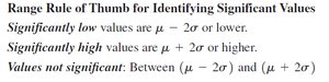
The Range Rule of Thumb helps identify significant values in a dataset:

• Significantly low values: $\mu - 2\sigma$ or lower

• Significantly high values: $\mu + 2\sigma$ or higher

• Values not significant: Between $\mu - 2\sigma$ and $\mu + 2\sigma$

Empirical Rule

For bell-shaped (normal) distributions:

• About 68% of values fall within 1 standard deviation of the mean.

• About 95% within 2 standard deviations.

• About 99.7% within 3 standard deviations.

Chebychev's Theorem

Applies to any data distribution, not just normal:

• At least $1 - \frac{1}{k^2}$ of values lie within $k$ standard deviations of the mean (for $k > 1$).

Comparison: The Empirical Rule is specific to normal distributions, while Chebychev's Theorem applies to all distributions.

Measures of Relative Standing (Position)

These measures describe the position of a value within a dataset.

• Standard Scores (z-scores): $z = \frac{x - \mu}{\sigma}$; measures how many standard deviations a value is from the mean.

• Percentile: The percentage of values below a given value $x$. Formula: $P = \frac{\#\text{ below } x}{n} \cdot 100\%$

• Finding x given Percentile Rank: $l = \frac{k}{100} \cdot n$

• Quartiles: Divide data into four equal parts.

• Five-Number Summary: Minimum, Q1, Median, Q3, Maximum.

• Boxplots: Visual representation of the five-number summary; modified boxplots highlight outliers.

• Outliers: Values more than 1.5 IQRs away from Q1 or Q3.

Example: If Q1 = 10, Q3 = 20, IQR = 10, then any value below $10 - 1.5 \times 10 = -5$ or above $20 + 1.5 \times 10 = 35$ is an outlier.