Statistical Inference and Hypothesis Testing: Concepts and Applications

Statistical Inference

Population and Sample

Statistical inference involves making conclusions about a population based on information obtained from a sample. The population is the entire group of interest, while a sample is a subset of the population used to draw conclusions due to practical constraints.

• Population: All elements of interest in a target group.

• Sample: Any subset of the population, ideally random and representative.

• Test Statistic: A value calculated from the sample data, used to make inferences about the population.

Example: Measuring stress levels in all seals in captivity should involve a representative sample, not just those from one location.

Hypothesis Testing

Purpose and Structure

Hypothesis testing is a formal procedure to determine if there is enough statistical evidence to support a specific belief about a population. It involves comparing two competing hypotheses:

• Null Hypothesis (H0): The default assumption (e.g., no effect, no difference).

• Alternative Hypothesis (HA): The claim we seek evidence for (e.g., there is an effect or difference).

Example: In a criminal trial, H0: The defendant is innocent; HA: The defendant is guilty.

Possible Outcomes and Errors

There are four possible outcomes in hypothesis testing, depending on the truth of H0 and the decision made:

	H0 is true	H0 is false
Do not reject H0	Correct decision	Type II error (β)
Reject H0	Type I error (α)	Correct decision

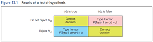
• Type I Error (α): Rejecting H0 when it is true (false positive).

• Type II Error (β): Not rejecting H0 when it is false (false negative).

• Power of a Test: Probability of correctly rejecting H0 when it is false (1 - β).

Significance Level and p-value

Alpha (α) and Decision Making

The significance level (α) is the threshold for deciding whether to reject H0. Common values are 0.05, 0.01, and 0.10. The p-value is the probability of observing data as extreme as, or more extreme than, the observed data if H0 is true.

• If p-value < α, reject H0.

• If p-value ≥ α, do not reject H0.

Example: If α = 0.05 and p-value = 0.03, we reject H0 with a 5% risk of a Type I error.

Statistical Distributions

Understanding Distributions

A statistical distribution describes the possible values for a variable and how often they occur. For example, rolling a fair die produces a uniform distribution where each outcome is equally likely.

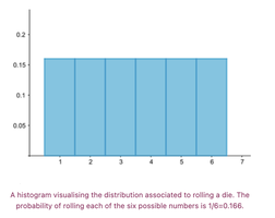
• Uniform Distribution: All outcomes are equally probable.

• Normal Distribution: Symmetrical, bell-shaped curve common in many natural phenomena.

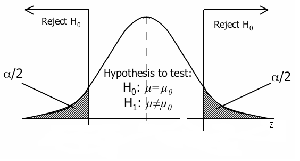
One-Tail and Two-Tail Tests

Test Directionality

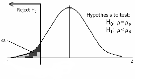
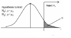
Hypothesis tests can be one-tailed or two-tailed depending on the research question:

• Left-tail test: Tests if the parameter is less than a value.

• Right-tail test: Tests if the parameter is greater than a value.

• Two-tail test: Tests if the parameter is different (either direction) from a value.

The Pearson (Chi-Squared) Test Statistic

Purpose and Types

The Pearson chi-squared test is used to compare observed frequencies with expected frequencies. There are two main types:

• Goodness of Fit Test: Tests if the distribution of a single categorical variable matches expectations.

• Test of Independence: Tests if two categorical variables are independent.

Chi-Squared Test Formula

The test statistic is calculated as:

$T = \sum\limits_{i=1}^k \frac{(O - E)^2}{E}$

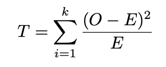
• O: Observed frequency

• E: Expected frequency

Goodness of Fit Example: Gold Lotto

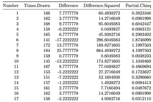
Suppose we want to test if a lottery is fair. The expected frequency for each number is calculated, and the observed frequencies are compared using the chi-squared formula. The partial calculations are shown in the table below:

Number	Times Drawn	Difference	Difference Squared	Partial ChiSq
1	166	7.7777778	60.4938272	0.3823346
2	162	3.7777778	14.2716049	0.0901919
3	168	9.7777778	95.6049383	0.6042472
...	...	...	...	...

Chi-Squared Distribution and Degrees of Freedom

The chi-squared distribution describes the probability of the test statistic under the null hypothesis. The shape depends on the degrees of freedom (df), which is typically the number of categories minus one.

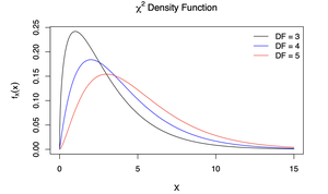
• Degrees of Freedom (df): Number of categories minus one (for goodness of fit).

Critical Values and Statistical Decision

To determine significance, compare the calculated test statistic to the critical value from the chi-squared table for the appropriate degrees of freedom and significance level (α). If the test statistic exceeds the critical value, reject H0.

• Example: For df = 44 and α = 0.05, the critical value is approximately 67.5. If the test statistic is 31, do not reject H0.

Pearson’s Chi-Square Test of Independence

Purpose and Application

This test determines if two categorical variables are independent. The expected frequency for each cell in a contingency table is calculated as:

$E_{ij} = \frac{(\text{Row Total})_i \times (\text{Column Total})_j}{\text{Grand Total}}$

• Null Hypothesis (H0): The variables are independent.

• Alternative Hypothesis (HA): The variables are not independent.

Example: Testing if students' favorite subjects are associated with their grade levels using a contingency table.

Summary and Takeaways

• Statistical inference allows us to draw conclusions about populations using samples.

• Hypothesis testing involves formulating null and alternative hypotheses, calculating a test statistic, and making a decision based on significance levels and p-values.

• Type I and Type II errors are important considerations in hypothesis testing.

• The chi-squared test is a key tool for analyzing categorical data, both for goodness of fit and independence.