Statistics Test 1 Review: Descriptive Statistics, Probability, and Distributions

Descriptive Statistics

Variables and Individuals

Descriptive statistics involve summarizing and organizing data to understand its main features. The two fundamental concepts are variables and individuals.

• Individual: The entity being measured or observed (e.g., a batch of pizza dough, a city, a person).

• Variable: A characteristic or property measured on individuals. Variables can be:

  • Qualitative (Categorical): No numeric value or intrinsic order (e.g., recipe type).

  • Quantitative (Numeric): Numeric values, which can be:

    • Discrete: Countable values, often integers (e.g., number of color blind men).

    • Continuous: Any value within a range (e.g., calcium concentration in water).

Types of Graphs for Data Visualization

Graphs are essential for visualizing data distributions and relationships. The choice of graph depends on the variable type.

• Frequency Distribution: Shows counts for each category or value.

• Relative Frequency Distribution: Shows proportions for each category or value.

• Pie Chart: Visualizes proportions of categorical data.

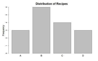
• Bar Graph: Compares frequencies or proportions for categorical data.

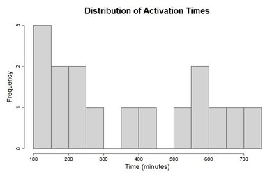
• Histogram: Displays frequency of numeric data grouped into intervals.

• Dotplot: Shows individual data points for small datasets.

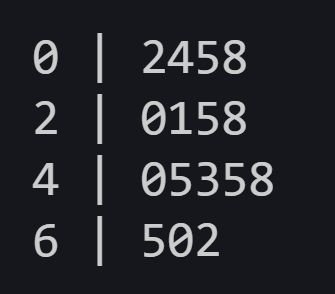
• Stemplot: Splits data into stems and leaves for quick visualization.

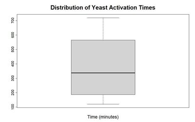
• Boxplot: Summarizes distribution using quartiles and highlights outliers.

Example: Distribution of Recipes (Bar Graph)

Example: Distribution of Activation Times (Histogram)

Example: Stemplot of Activation Times

Example: Boxplot of Yeast Activation Times

Describing Distributions

To describe a distribution, consider:

• Center: Mean, median, mode

• Spread: Range, interquartile range (IQR), standard deviation (SD)

• Shape: Symmetry, skewness, modality (number of peaks), outliers

Example: Water Hardness (Calcium Concentration)

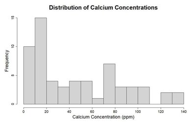
• Individuals: Cities

• Variable: Calcium concentration (continuous, numeric)

• Distribution: Skewed right, possible outliers, unimodal

Probability Foundations

Basic Definitions

• Sample Space (S): All possible outcomes of a random experiment.

• Event: Any subset of the sample space.

• Probability Model: Assigns probabilities to outcomes/events.

Probability Definitions

• Symmetry Definition: If all outcomes are equally likely, $P(A) = \frac{\text{Number of outcomes in } A}{\text{Total number of outcomes}}$

• Frequentist Definition: Probability is the long-run proportion of times an event occurs in repeated trials.

Probability Rules

• Addition Rule (Special): For mutually exclusive events, $P(A \text{ or } B) = P(A) + P(B)$

• Addition Rule (General): $P(A \text{ or } B) = P(A) + P(B) - P(A \text{ and } B)$

• Complement Rule: $P(A^c) = 1 - P(A)$

Venn Diagrams

Venn diagrams visually represent relationships between events in a sample space, aiding in understanding probability rules.

Independence and Conditional Probability

• Independent Events: $P(A \text{ and } B) = P(A) \times P(B)$

• Conditional Probability: $P(A|B) = \frac{P(A \text{ and } B)}{P(B)}$

Contingency Tables

Contingency tables display frequencies for combinations of two categorical variables. Marginal totals are row/column sums; the grand total is the sum of all cells.

Age Group	Some H.S.	High School	Some Uni.	University	Total
25-34	27	82	43	48	200
35-44	50	19	56	75	200
45-54	52	88	26	34	200
55-64	71	83	20	26	200
65+	101	59	20	20	200
Total	301	331	165	203	1000

Counting Rules

• Permutations: Number of ways to arrange n objects: $n!$

• Combinations: Number of ways to choose r objects from n: $\binom{n}{r} = \frac{n!}{r!(n-r)!}$

Discrete Random Variables

Discrete Distributions

Discrete random variables take on countable values. Their distributions specify the probability for each possible value.

• Mean (Expected Value): $\mu = \sum x_i p_i$

• Standard Deviation: $\sigma = \sqrt{\sum (x_i - \mu)^2 p_i}$

Binomial Distribution

• Models the number of successes in n independent trials, each with probability p of success.

• Probability: $P(X = k) = \binom{n}{k} p^k (1-p)^{n-k}$

• Mean: $\mu = np$

• Standard Deviation: $\sigma = \sqrt{np(1-p)}$

Poisson Distribution

• Models the number of events in a fixed interval, given a known average rate.

• Probability: $P(X = k) = \frac{\lambda^k e^{-\lambda}}{k!}$

• Mean and SD: $\mu = \sigma = \lambda$

Continuous Random Variables

Probability Density Functions (PDFs)

• Probability is the area under the density curve over an interval.

• Probability of a single value is zero.

• Mean and SD are defined similarly to discrete variables, using integrals.

Exponential Distribution

• Models time between events in a Poisson process.

• PDF: $f(x) = \lambda e^{-\lambda x}$ for $x \geq 0$

• Mean: $\mu = 1/\lambda$

• SD: $\sigma = 1/\lambda$

Normal Distribution

• Symmetric, bell-shaped distribution defined by mean $\mu$ and standard deviation $\sigma$.

• PDF: $f(x) = \frac{1}{\sigma \sqrt{2\pi}} e^{-\frac{(x-\mu)^2}{2\sigma^2}}$

• Probabilities are found using standard normal tables or functions (e.g., pnorm, qnorm).

Example: Distribution of Calcium Concentrations (Histogram)

Empirical Rule

• For normal distributions:

  • ~68% of data within 1 SD of mean

  • ~95% within 2 SD

  • ~99.7% within 3 SD

Summary Table: Graph Types and Their Uses

Graph Type	Variable Type	Main Use
Bar Graph	Categorical	Compare frequencies/proportions
Pie Chart	Categorical	Show proportions
Histogram	Numeric (Continuous/Discrete)	Show distribution shape
Dotplot	Numeric (Small datasets)	Show individual values
Stemplot	Numeric (Small datasets)	Quick visualization
Boxplot	Numeric	Summarize spread, center, outliers

Additional info: Some explanations and table entries were expanded for completeness and clarity based on standard statistics curriculum.