Statistics Test Review: Visual Data Interpretation and Descriptive Statistics

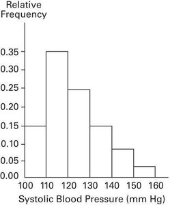
Q7. Approximately what percentage of the people aged 25-40 had a systolic blood pressure reading between 110 and 139 mm Hg inclusive?

Background

Topic: Interpreting Histograms and Relative Frequency

This question tests your ability to read a relative frequency histogram and estimate the proportion (percentage) of a population that falls within a specified range of values.

Key Terms and Concepts:

• Relative Frequency: The proportion of the total number of data points that fall within a particular class interval.

• Histogram: A graphical representation of the distribution of numerical data, where the area of each bar is proportional to the frequency of items in each interval.

• Percentage: To convert a relative frequency to a percentage, multiply by 100.

Step-by-Step Guidance

1. Identify the class intervals on the x-axis that fall between 110 and 139 mm Hg (inclusive). These are the bars labeled 110-120, 120-130, and 130-140.

2. Read the relative frequency (height) of each relevant bar from the histogram. Write down the relative frequency for each interval within the specified range.

3. Add the relative frequencies for all the intervals that fall within 110 to 139 mm Hg.

4. Convert the sum of the relative frequencies to a percentage by multiplying by 100.

5. Check that you have included all intervals that are within the specified range and none outside it.

Try solving on your own before revealing the answer!

Final Answer: 75%

By summing the relative frequencies for the intervals 110-120, 120-130, and 130-140, you get 0.35 + 0.25 + 0.15 = 0.75. Multiplying by 100 gives 75%. This means approximately 75% of people aged 25-40 had a systolic blood pressure reading between 110 and 139 mm Hg inclusive.

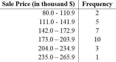
Q13. The frequency distribution below summarizes the home sale prices in the city of Summerhill for the month of June. Determine the class width.

Background

Topic: Frequency Distributions and Class Width

This question tests your understanding of how to determine the class width from a frequency distribution table.

Key Terms and Formula:

• Class Width: The difference between the lower boundaries (or upper boundaries) of two consecutive classes in a frequency distribution.

• Formula:

$\text{Class Width} = \text{Lower limit of second class} - \text{Lower limit of first class}$

Step-by-Step Guidance

1. Identify the lower limit of the first class and the lower limit of the second class from the table.

2. Subtract the lower limit of the first class from the lower limit of the second class to find the class width.

3. Check that the class width is consistent across all classes in the table.

Try solving on your own before revealing the answer!

Final Answer: 31.0 (in thousands $)

The class width is found by subtracting 80.0 from 111.0, which gives 31.0. This width is consistent for all classes in the table.

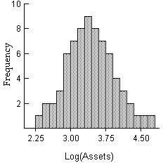
Q14. The histogram below shows the distribution of the assets (in millions of dollars) of 71 companies. Does the distribution appear to be normal?

Background

Topic: Shape of Distributions (Normality)

This question tests your ability to visually assess whether a distribution is approximately normal by looking at a histogram.

Key Terms:

• Normal Distribution: A symmetric, bell-shaped distribution where most of the data clusters around the mean.

• Histogram: A graphical representation of the distribution of data.

Step-by-Step Guidance

1. Look for symmetry in the histogram. A normal distribution should be roughly symmetric about the center.

2. Check if the histogram has a single peak (unimodal) and tails that decrease gradually on both sides.

3. Assess whether the frequencies decrease as you move away from the center in both directions.

4. Consider if there are any significant outliers or skewness that would indicate a non-normal distribution.

Try solving on your own before revealing the answer!

Final Answer: Yes, it appears to be normal.

The histogram is roughly symmetric and bell-shaped, with most data clustered around the center and frequencies tapering off on both sides, which is characteristic of a normal distribution.

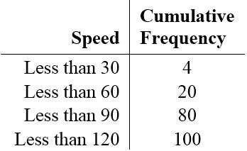
Q9. Create a cumulative frequency chart for the given frequency distribution.

Background

Topic: Cumulative Frequency

This question tests your ability to construct a cumulative frequency table from a frequency distribution.

Key Terms and Concepts:

• Cumulative Frequency: The sum of the frequencies for all classes up to and including the current class.

• Frequency Distribution: A table that shows the number of occurrences for each class interval.

Step-by-Step Guidance

1. Start with the first class interval and record its frequency as the first cumulative frequency.

2. For each subsequent class, add its frequency to the cumulative frequency of the previous class.

3. Continue this process for all class intervals in the table.

4. Check that the final cumulative frequency equals the total number of data points.

Try solving on your own before revealing the answer!

Final Answer:

The cumulative frequency chart is:

Speed	Cumulative Frequency
Less than 30	4
Less than 60	20
Less than 90	80
Less than 120	100

This table shows the running total of frequencies up to each speed class.

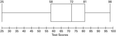
Q16. Construct a boxplot for the given data. Include the values of the 5-number summary. The test scores of 40 students are listed below.

Background

Topic: Boxplots and Five-Number Summary

This question tests your ability to construct a boxplot and identify the five-number summary (minimum, Q1, median, Q3, maximum) from a data set.

Key Terms and Concepts:

• Boxplot: A graphical summary of data showing the minimum, first quartile (Q1), median, third quartile (Q3), and maximum.

• Five-Number Summary: Minimum, Q1, Median, Q3, Maximum.

Step-by-Step Guidance

1. Order the data from smallest to largest.

2. Identify the minimum and maximum values in the data set.

3. Find the median (the middle value or average of the two middle values).

4. Determine the first quartile (Q1) and third quartile (Q3) by finding the medians of the lower and upper halves of the data.

5. Draw a boxplot using these five values, with a box from Q1 to Q3, a line at the median, and "whiskers" extending to the minimum and maximum.

Try solving on your own before revealing the answer!

Final Answer:

The five-number summary is: Minimum = 25, Q1 = 58, Median = 72, Q3 = 81, Maximum = 98. The boxplot visually displays these values, showing the spread and center of the data.