Statistics Unit 1: Data Collection, Summarization, and Numerical Description

Data Collection and Types of Data

Population, Sample, and Variables

Understanding the distinction between populations and samples is fundamental in statistics. A population is the entire group of individuals or items of interest, while a sample is a subset selected from the population. Parameters are numerical summaries describing populations, whereas statistics describe samples.

• Descriptive statistics: Methods for summarizing and organizing data.

• Inferential statistics: Methods for making predictions or inferences about a population based on sample data.

• Variables: Characteristics or properties that can take on different values.

• Quantitative variables: Numeric values (discrete or continuous).

• Qualitative (categorical) variables: Non-numeric categories or groups.

Explanatory variables are used to explain or predict changes in response variables.

Study Designs and Sampling Methods

Statistical studies can be observational or experimental. Observational studies include cross-sectional, case-control, and cohort designs, while experiments may be completely randomized or use matched-pairs designs. Proper sampling is crucial to avoid bias and ensure representativeness.

• Sampling schemes: Simple random, stratified, cluster, convenience, multistage.

• Sources of bias: Sampling bias, nonresponse bias, response bias, undercoverage.

• Open vs. closed questions: Open questions allow free responses; closed questions provide fixed options.

• Sampling errors: Errors due to the process of selecting a sample.

• Non-sampling errors: Errors not related to sampling, such as data entry mistakes.

In experiments, terms such as experimental unit/subject, factor, and treatment are used. The placebo effect, blinding, and replication are important for validity.

Organizing and Summarizing Data

Raw Data and Frequency Distributions

Raw data can be organized into frequency distributions, which summarize data into classes or categories. Key terms include class width, class limits, class midpoints, frequency, relative frequency, and cumulative frequency.

• Qualitative data graphs: Bar graph, Pareto chart, side-by-side bar graph, pie chart.

• Quantitative data graphs: Histogram, dot plot, stem-and-leaf plot, time-series graph, boxplot.

• Distribution shapes: Symmetric, uniform, bell-shaped, skewed left, skewed right.

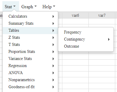
Statistical software such as StatCrunch can be used to construct these graphs and tables.

Numerically Summarizing Data

Measures of Center

Measures of center describe the typical value in a data set. The most common measures are the mean, median, and mode.

• Mean (arithmetic mean): The average value. For a sample: $\bar{x} = \frac{\sum x_i}{n}$; for a population: $\mu = \frac{\sum x_i}{N}$.

• Weighted mean: $\bar{x}_w = \frac{\sum (w_i \cdot x_i)}{\sum w_i}$

• Median: The middle value when data are ordered. If n is odd, median is the $\frac{n+1}{2}$th value; if n is even, median is the mean of the $\frac{n}{2}$th and $\frac{n}{2}+1$th values.

• Mode: The most frequently occurring value(s).

Data sets may be no mode, bimodal, or multimodal. The mean and standard deviation can be calculated for both populations and samples, with sample statistics often being resistant to outliers.

Measures of Dispersion

Measures of dispersion describe the spread of data values.

• Range: Difference between largest and smallest values. $\text{Range} = \text{max} - \text{min}$

• Variance (sample): $s^2 = \frac{\sum (x_i - \bar{x})^2}{n-1}$

• Standard deviation (sample): $s = \sqrt{s^2} = \sqrt{\frac{\sum (x_i - \bar{x})^2}{n-1}}$

• Variance (population): $\sigma^2 = \frac{\sum (x_i - \mu)^2}{N}$

• Standard deviation (population): $\sigma = \sqrt{\sigma^2} = \sqrt{\frac{\sum (x_i - \mu)^2}{N}}$

• Interquartile range (IQR): $\text{IQR} = Q_3 - Q_1$

The Empirical Rule

The Empirical Rule applies to bell-shaped (normal) distributions and describes the proportion of data within certain standard deviations of the mean:

• Approximately 68% within 1 standard deviation ($\mu \pm 1\sigma$)

• Approximately 95% within 2 standard deviations ($\mu \pm 2\sigma$)

• Approximately 99.7% within 3 standard deviations ($\mu \pm 3\sigma$)

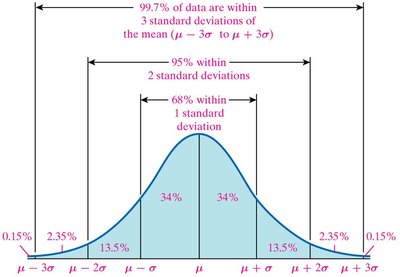
For sample data, use $\bar{x}$ and $s$ in place of $\mu$ and $\sigma$.

Measures of Position and Outliers

Measures of position help describe the relative standing of a data value within a data set.

• z-score: Indicates how many standard deviations a value is from the mean. For a sample: $z = \frac{x - \bar{x}}{s}$; for a population: $z = \frac{x - \mu}{\sigma}$

• Percentiles: The kth percentile is a value below which k percent of the data fall.

• Quartiles: Divide data into four equal parts. $Q_1$ is the median of the lower half, $Q_2$ is the median, $Q_3$ is the median of the upper half.

• Five-number summary: Minimum, $Q_1$, median ($Q_2$), $Q_3$, maximum.

• Interquartile Range (IQR): $\text{IQR} = Q_3 - Q_1$

To identify outliers:

1. Find $Q_1$ and $Q_3$.

2. Compute IQR.

3. Calculate fences: Lower fence = $Q_1 - 1.5 \times \text{IQR}$; Upper fence = $Q_3 + 1.5 \times \text{IQR}$.

4. Values outside these fences are considered outliers.

Boxplots can be used to visually identify outliers using these fences.

Additional info:

• Statistical software such as StatCrunch provides menu options for constructing frequency tables, graphs, and summary statistics, as shown in the included image.

• All formulas are provided in LaTeX format for clarity and ease of reference.