STT 2810 Final Exam Study Guide: Key Concepts and Formulas

Symbols and Formulas in Statistics

Sample and Population Symbols

Understanding the notation for sample and population statistics is fundamental in statistics. These symbols are used to distinguish between values calculated from a sample and those from the entire population.

• Sample Mean: \( \bar{x} \)

• Population Mean: \( \mu \)

• Sample Standard Deviation: \( s \)

• Population Standard Deviation: \( \sigma \)

Example: If a sample of exam scores has a mean of 75, it is denoted as \( \bar{x} = 75 \). If the population mean is 80, it is \( \mu = 80 \).

Least Squares Regression Line

The least squares regression line is used to model the relationship between two quantitative variables. The formula is:

• \( \hat{y} = b_0 + b_1x \)

• \( b_0 \): y-intercept

• \( b_1 \): slope

• \( \hat{y} \): predicted y value

R2: Represents the percentage of variation in y explained by changes in x.

Confidence Intervals and Sampling Distributions

Confidence Interval for One Population Mean (Sigma Unknown)

When the population standard deviation is unknown, use the t-distribution:

• \( \bar{x} \pm t^* \frac{s}{\sqrt{n}} \)

• t*: Critical value from t-distribution

• Standard Error: \( \frac{s}{\sqrt{n}} \)

Confidence Interval for One Population Proportion

For proportions, use the z-distribution:

• \( \hat{p} \pm z^* \sqrt{\frac{\hat{p}(1-\hat{p})}{n}} \)

• z*: Critical value from z-distribution

• Standard Error: \( \sqrt{\frac{\hat{p}(1-\hat{p})}{n}} \)

Sampling Distribution of Sample Means

The sampling distribution of sample means describes how the mean of samples varies:

• \( \bar{x} \sim N\left(\mu, \frac{\sigma}{\sqrt{n}}\right) \)

• Mean: \( \mu \)

• Standard Deviation: \( \frac{\sigma}{\sqrt{n}} \)

Sampling Distribution of Sample Proportions

Describes the distribution of sample proportions:

• \( \hat{p} \sim N\left(p, \sqrt{\frac{p(1-p)}{n}}\right) \)

• Mean: \( p \)

• Standard Deviation: \( \sqrt{\frac{p(1-p)}{n}} \)

Margin of Error for Difference in Two Population Proportions

Used to construct a confidence interval for the difference between two proportions:

• \( (\hat{p}_1 - \hat{p}_2) \pm z^* \sqrt{\frac{\hat{p}_1(1-\hat{p}_1)}{n_1} + \frac{\hat{p}_2(1-\hat{p}_2)}{n_2}} \)

Errors in Hypothesis Testing

Type I and Type II Errors

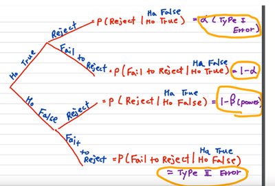
In hypothesis testing, errors can occur when making decisions about the null hypothesis (H0) and alternative hypothesis (Ha). The following table summarizes the conditional probabilities associated with these errors:

Decision	Truth	Probability	Term
Reject H0	H0 True	\( \alpha \)	Type I Error
Fail to Reject H0	H0 True	\( 1-\alpha \)	Correct Decision
Reject H0	H0 False	\( 1-\beta \)	Power
Fail to Reject H0	H0 False	\( \beta \)	Type II Error

Type I Error (\( \alpha \)): Rejecting H0 when it is true. Type II Error (\( \beta \)): Failing to reject H0 when it is false. Power (\( 1-\beta \)): Probability of correctly rejecting H0 when it is false.

Describing and Displaying Data

5 W's and 1 H

To fully describe a dataset, answer the following:

• Who: The subjects or cases

• What: The variables measured

• When: The time of data collection

• Where: The location of data collection

• Why: The purpose of the study

• How: The method of data collection

Marginal Distributions and Contingency Tables

Marginal distributions summarize the totals for each category in a contingency table:

• Formula: Row or column total / overall total

• Application: Used when interested in one group out of everyone

Dot Plots and Skewness

Dot plots help visualize the distribution of data:

• Skewed: Use median and IQR

• Symmetric: Use mean and standard deviation

• Skewed Left: Mean < Median

• Skewed Right: Mean > Median

Summary Statistics and Boxplots

Summary statistics include mean, standard deviation, IQR, quartiles, min, max, and median. Boxplots visually compare medians, ranges, and IQRs.

• 5 Number Summary: Min, Q1, Median, Q3, Max

• Boxplot Comparison: Consider context; a lower median may imply faster/slower times depending on the variable.

Shift/Scale Data

Scaling (multiplying/dividing) changes all values in a dataset. For example, reducing speed by 9% means multiplying by 0.91.

Normal Model and Z-Scores

Normal Calculator and Percentiles

Use a normal calculator to find probabilities or percentiles by adjusting mean and standard deviation.

• Z-score: Tells how many standard deviations a value is from the mean.

• Formula: \( z = \frac{x - \mu}{\sigma} \)

Scatterplots, Correlation, and Regression

Scatterplot Description

Describe form, direction, and strength:

• Form: Linear or nonlinear

• Direction: Positive or negative

• Strength: Strong, moderate, weak

Correlation (r)

Correlation measures linear association:

• \( r \) ranges from -1 to 1

• \( r = 0 \): No linear relationship

• \( r = 1 \): Perfect positive linear

• \( r = -1 \): Perfect negative linear

• Correlation has no units and is unaffected by shifting/scaling

Residual Plots

A residual plot is appropriate if it is not curved or does not show changing spread. The least squares regression line minimizes the sum of squared residuals.

Regression Line Interpretation

The slope indicates the average change in y for each unit increase in x.

• Interpretation: For every one unit increase in x, y increases/decreases by the slope.

R2 Interpretation

R2 is the percent of variation in y explained by x.

Finding Actual y Value

Given predicted y and residual:

• \( \text{Residual} = \text{Actual y} - \text{Predicted y} \)

• \( \text{Actual y} = \text{Residual} + \text{Predicted y} \)

Sampling and Surveys

Sample, Sampling Frame, and Population

Definitions:

• Sample: Subset of the population

• Sampling Frame: List from which the sample is drawn

• Population: Entire group of interest

Sampling Methods

• Random: Stratified, Cluster, Systematic, Simple Random Sample

• Not Random: Voluntary Response, Convenience Sampling

Bias

Voluntary response bias occurs when participants self-select into the sample.

Probability and Random Variables

Sample Space and Probability Models

Sample space lists all possible outcomes. A probability model is legitimate if probabilities sum to 1.

Probability Rules

• Complement Rule: \( P(A^c) = 1 - P(A) \)

• Multiplication Rule (Independent Events): \( P(A \text{ and } B) = P(A)P(B) \)

• General Addition Rule: \( P(A \text{ or } B) = P(A) + P(B) - P(A \text{ and } B) \)

Conditional Probability

Probability of an event given another event has occurred.

Tree Diagrams

Tree diagrams help visualize conditional probabilities and sample spaces.

Random Variables

Define random variables, assign probabilities, and calculate expected value and standard deviation.

• Expected Value: \( E(X) = \sum x_i P(x_i) \)

• Standard Deviation: \( \sqrt{\sum (x_i - E(X))^2 P(x_i)} \)

Mean and Standard Deviation of X - Y

• Mean: \( \mu_{X-Y} = \mu_X - \mu_Y \)

• Standard Deviation: \( \sigma_{X-Y} = \sqrt{\sigma_X^2 + \sigma_Y^2} \)

Sampling Distribution for Proportions and Means

Conditions for Normal Model (Sample Proportions)

• Random

• 10% Condition

• Success/Failure Condition

Sample Size for Confidence Interval

Use \( p = 0.5 \) if not given. Find z* using normal calculator.

Hypothesis Testing and Confidence Intervals

Null and Alternative Hypotheses

• Null: Always has an equal sign

• Alternative: Not equal, greater, or less

Interpreting Type I and II Errors

Type I: False positive; Type II: False negative.

Confidence Interval for Difference in Two Proportions

Use sample proportions and sizes to find successes.

Interpreting p-value

If null is true, p-value is the chance of seeing the observed difference or larger by natural sampling variation.

Confidence Interval for One Mean

Use t-distribution; compute lower and upper limits.

Critical Value of t

Find using t-distribution calculator with appropriate degrees of freedom.

Interpreting Confidence Interval for Difference in Means

• (-, -): Second group larger

• (+, +): First group larger

• (-, +): Mixed

Additional info: These notes expand on brief exam review points, providing definitions, formulas, and context for each topic. The included tree diagram visually clarifies conditional probabilities and error types in hypothesis testing.