Study Guide: Normal Probability Distributions in Statistics

Normal Probability Distributions

Introduction to the Normal Distribution

The normal distribution is a fundamental concept in statistics, describing a continuous probability distribution that is symmetric and bell-shaped. It is widely used in the health sciences and other fields to model real-world phenomena.

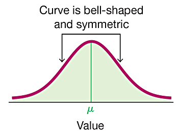
• Definition: A continuous random variable has a normal distribution if its graph is symmetric and bell-shaped.

• Key Properties: The mean, median, and mode are all equal; the curve is symmetric about the mean; and the total area under the curve is 1.

• Density Curve: The graph of any continuous probability distribution is called a density curve, and the area under the curve represents probability.

The Standard Normal Distribution

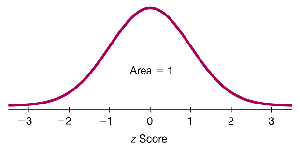
The standard normal distribution is a special case of the normal distribution with a mean of 0 and a standard deviation of 1. It is used to calculate probabilities and z scores for various regions under the curve.

• Notation: The variable z represents the number of standard deviations a value is from the mean.

• Area and Probability: The area under the curve corresponds to probability, and the total area is 1.

Finding Probabilities Using z Scores

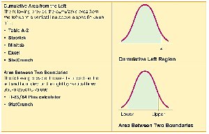
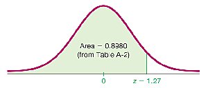
Probabilities for the normal distribution are found by calculating the area under the curve for a given z score. This can be done using statistical tables or technology.

• Left of z: Probability that a value is less than a given z score.

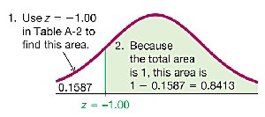
• Right of z: Probability that a value is greater than a given z score.

• Between z values: Probability that a value falls between two z scores.

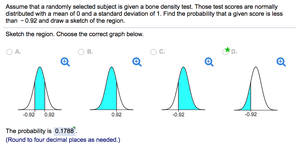
Examples: Bone Density Test

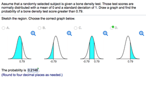
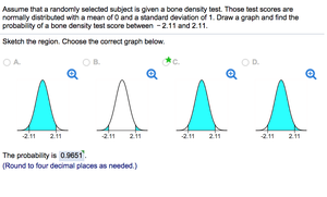
Bone density test scores are often modeled using the standard normal distribution. The probability of a score less than or greater than a certain value can be found using z scores and area under the curve.

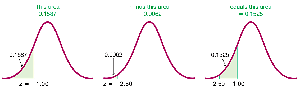
• Example: Probability that a bone density test score is less than 1.27.

• Example: Probability that a score is above -1.00.

• Example: Probability that a score is between -1.00 and -2.50.

Notation and Critical Values

Statistical notation is used to represent probabilities and critical values in the normal distribution.

• P(a < z < b): Probability that z is between a and b.

• P(z > a): Probability that z is greater than a.

• P(z < a): Probability that z is less than a.

• Critical Value: A z score on the borderline separating significantly low or high values. Notation: zα denotes the z score with an area of α to its right.

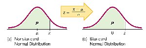
Converting Nonstandard Normal Distributions

When the mean and standard deviation are not 0 and 1, values can be converted to z scores using the formula:

• Conversion Formula: $z = \frac{x - \mu}{\sigma}$

• Application: Allows any normal distribution to be standardized for probability calculations.

Example: Heights of Men and Showerhead Design

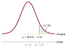
Heights of men are normally distributed. To find the proportion taller than a certain height, convert the value to a z score and find the area to the right.

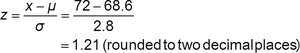
• Given: Mean = 68.6 in., σ = 2.8 in., height = 72 in.

• Step 1: Convert 72 in. to z score: $z = \frac{72 - 68.6}{2.8} = 1.21$

• Step 2: Find area to the right of z = 1.21.

• Result: About 11% of men are taller than 72 in.

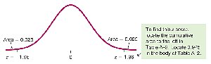
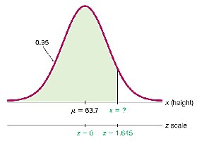
Finding Values from Known Areas

When the area (probability or percentage) is known, the corresponding value can be found using the z score and conversion formula.

• Procedure: Sketch the curve, identify the region, use Table A-2 or technology to find the z score, then convert to x using $x = \mu + z\sigma$.

• Percentiles: The value corresponding to a given percentile can be found using the same method.

Sampling Distributions and Estimators

A sampling distribution is the distribution of a statistic (such as sample mean or proportion) when all possible samples of a given size are taken from a population.

• Sample Proportions: Tend to be normally distributed; mean equals the population mean.

• Unbiased Estimators: Statistics that target the population parameter (mean, proportion, variance).

• Biased Estimators: Statistics that do not target the population parameter (median, range, sample standard deviation).

The Central Limit Theorem

The central limit theorem states that the distribution of sample means approaches a normal distribution as the sample size increases, regardless of the population's distribution, provided n > 30 or the population is normal.

• Application: Allows use of normal distribution for inference about sample means.

• Notation: $\mu_{\bar{x}} = \mu$, $\sigma_{\bar{x}} = \frac{\sigma}{\sqrt{n}}$

Example: Safe Loading of Elevators

To assess elevator safety, calculate the probability that the mean weight of 27 randomly selected males exceeds a threshold using the normal distribution and central limit theorem.

• Step 1: Convert individual weight to z score.

• Step 2: For sample mean, use $\sigma_{\bar{x}} = \frac{\sigma}{\sqrt{n}}$.

• Result: Probability of exceeding weight threshold is extremely high, indicating risk.

Assessing Normality

To determine if data are from a normal distribution, use visual inspection, outlier identification, and normal quantile plots.

• Histogram: Should be bell-shaped and symmetric.

• Outliers: More than one outlier suggests non-normality.

• Normal Quantile Plot: Points should lie close to a straight line without systematic patterns.

Summary Table: Key Formulas and Concepts

Concept	Formula	Application
Standard Normal z Score	$z = \frac{x - \mu}{\sigma}$	Convert any value to standard normal
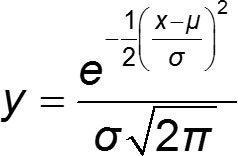
Normal Distribution PDF	$y = \frac{e^{-\frac{1}{2}\left(\frac{x-\mu}{\sigma}\right)^2}}{\sigma\sqrt{2\pi}}$	Probability density function
Sample Mean Distribution	$\mu_{\bar{x}} = \mu$, $\sigma_{\bar{x}} = \frac{\sigma}{\sqrt{n}}$	Central Limit Theorem

Additional info:

• All examples and images are directly relevant to the explanation of normal probability distributions, z scores, and their applications in statistics.

• Critical values and percentiles are important for hypothesis testing and statistical inference.

• Assessing normality is essential for determining the appropriateness of statistical methods.