Study Guide: The Normal Probability Distributions in Introductory Statistics

The Normal Probability Distributions

Introduction to Normal Distributions

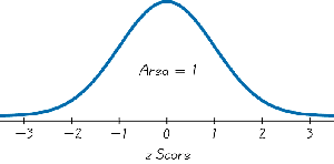
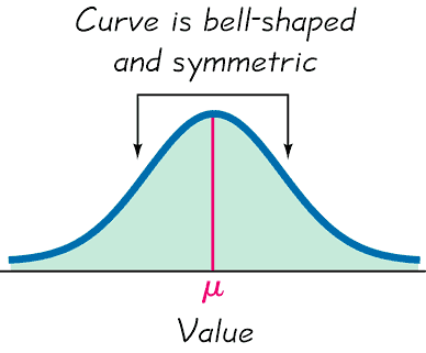
The normal distribution is a fundamental concept in statistics, describing a continuous random variable whose values are distributed in a symmetric, bell-shaped curve. This distribution is widely used due to its natural occurrence in many real-world phenomena and its mathematical properties.

• Definition: A normal distribution is a probability distribution with a graph that is symmetric and bell-shaped, characterized by its mean (μ) and standard deviation (σ).

• Standard Normal Distribution: A special case where the mean is 0 and the standard deviation is 1.

• Density Curve: The graph of any continuous probability distribution, with total area under the curve equal to 1.

Mathematical Equation of the Normal Distribution

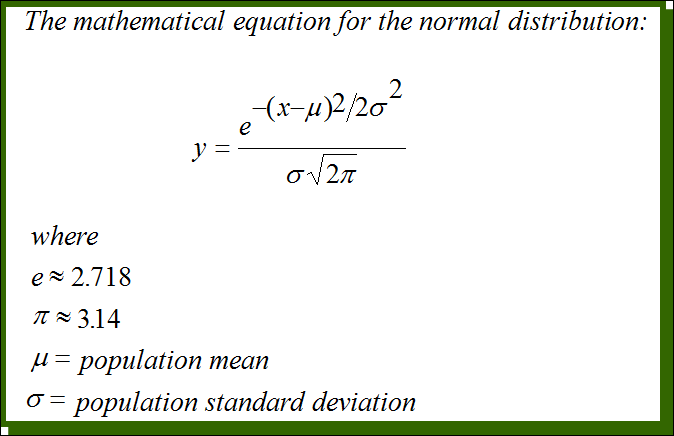
The normal distribution can be described mathematically by the following equation:

• Formula: $y = \frac{e^{-((x-\mu)^2)/(2\sigma^2)}}{\sigma \sqrt{2\pi}}$

• Parameters:

  • μ: Population mean

  • σ: Population standard deviation

  • e: Euler's number (≈ 2.718)

  • π: Pi (≈ 3.14)

Properties of Normal Distributions

• Symmetry: The curve is symmetric about the mean.

• Bell Shape: The distribution is bell-shaped, with most values clustering around the mean.

• Area Under Curve: The total area under the density curve is 1, representing the total probability.

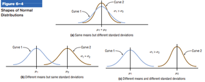
• Infinitely Many Distributions: There are infinitely many normal distributions, each defined by its own mean and standard deviation.

Uniform Distribution

Definition and Properties

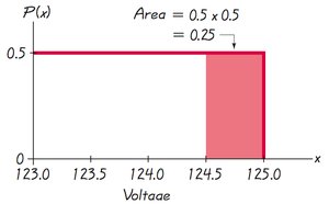
The uniform distribution is another type of continuous probability distribution where all values within a certain range are equally likely. Its graph is rectangular, and the area under the curve represents probability.

• Definition: A continuous random variable has a uniform distribution if its values are spread evenly over the range of possible values.

• Area Calculation: Probabilities are found by calculating the area of the rectangle: Area = height × width

• Total Area: The area under the graph is always 1.

Density Curves and Probability

Concepts and Examples

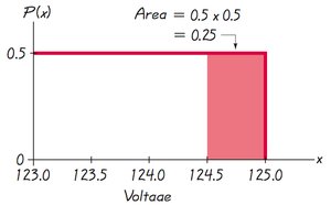
• Density Curve: Represents the probability distribution of a continuous random variable.

• Area-Probability Correspondence: The area under the curve for a given interval corresponds to the probability of the variable falling within that interval.

Standard Normal Distribution and Z Scores

Finding Probabilities Using Z Scores

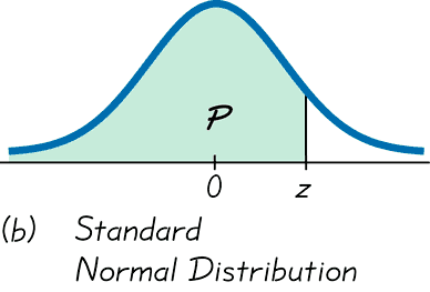
The standard normal distribution is used to find probabilities associated with z scores, which measure how many standard deviations a value is from the mean.

• Z Score: $z = \frac{x - \mu}{\sigma}$

• Notation:

  • $P(a < z < b)$: Probability z is between a and b

  • $P(z > a)$: Probability z is greater than a

  • $P(z < a)$: Probability z is less than a

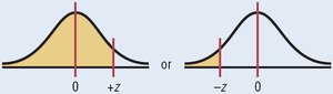
• Finding Probabilities:

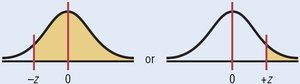
  • To the right of a z score: Subtract the area to the left from 1.

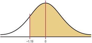
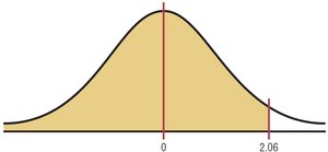
  • To the left of a z score: Use the area given in the table.

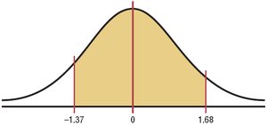
  • Between two z scores: Subtract the area for the lower z score from the area for the higher z score.

Applications of Normal Distributions

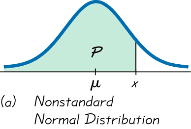
Standardizing Nonstandard Normal Distributions

When working with normal distributions that do not have a mean of 0 or a standard deviation of 1, values can be converted to z scores to use the standard normal distribution.

• Conversion Formula: $z = \frac{x - \mu}{\sigma}$

• Purpose: Allows comparison and calculation of probabilities using the standard normal table.

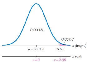
Example: Tall Clubs International

• Problem: Find the percentage of women at least 70 inches tall, given mean = 63.8 inches, σ = 2.6 inches.

• Steps:

  1. Convert x to z-score: $z = \frac{70 - 63.8}{2.6} = 2.38$

  2. Find area to the right of z = 2.38: 1 – 0.9913 = 0.0087

  3. Conclusion: About 0.87% of women meet the requirement.

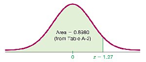
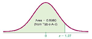
Example: Bone Density Test

• Problem: Find the probability that a randomly selected adult has a bone density test score less than 1.27.

• Solution: Area to the left of z = 1.27 is 0.8980, so the probability is 0.8980.

Example: Newspaper Recycling

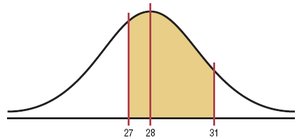
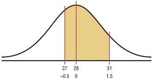
• Problem: Find the probability that a household generates between 27 and 31 pounds of newspaper per month, given mean = 28, σ = 2.

• Steps:

  1. Find z scores: $z_{27} = \frac{27 - 28}{2} = -0.5$, $z_{31} = \frac{31 - 28}{2} = 1.5$

  2. Find area between z = -0.5 (0.3085) and z = 1.5 (0.9332): 0.9332 – 0.3085 = 0.6247

  3. Conclusion: Probability is 62%.

Finding Z Scores from Probabilities

Percentiles and Critical Values

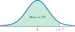
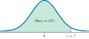
• Percentile: The z score corresponding to a given percentile can be found using the standard normal table.

• Example: The z score for the 95th percentile is approximately 1.645.

• Critical Value: For the standard normal distribution, a critical value is a z score on the borderline separating significantly low or high values. Notation: $z_\alpha$ denotes the z score with an area of α to its right.

Example: Aircraft Cabin Design

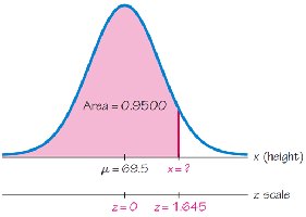
• Problem: What ceiling height allows 95% of men to stand without bumping their heads? Mean = 69.5 inches, σ = 2.4 inches.

• Solution: Find z = 1.645 for 95th percentile, then solve for x: $x = \mu + z \sigma = 69.5 + 1.645 \times 2.4 = 73.45$ inches

Example: Finding Critical Values

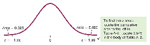
• Problem: Find the value of $z_{0.025}$.

• Solution: $z_{0.025} = 1.96$ (area of 0.025 to its right, cumulative left area of 0.975).

Summary Table: Normal Distribution Concepts

Concept	Definition	Formula
Normal Distribution	Symmetric, bell-shaped curve	$y = \frac{e^{-((x-\mu)^2)/(2\sigma^2)}}{\sigma \sqrt{2\pi}}$
Standard Normal Distribution	Normal distribution with μ = 0, σ = 1	$z = \frac{x - \mu}{\sigma}$
Uniform Distribution	All values equally likely within range	Area = height × width
Percentile	Value below which a percentage of data falls	Use z table
Critical Value	Z score separating significant values	$z_\alpha$

Additional info: All examples and images are directly relevant to the explanation of normal probability distributions, z scores, and their applications in introductory statistics.