Summarising Data: Numerical Methods in Statistics

Measures of Variability

Interquartile Range (IQR)

The interquartile range (IQR) is a measure of variability that focuses on the middle 50% of the data, reducing the influence of extreme values. It is calculated as the difference between the third quartile (Q3) and the first quartile (Q1):

• Formula: $IQR = Q_3 - Q_1$

• Advantages: Easy to interpret, not influenced by extreme values.

• Disadvantage: Only considers the middle 50% of the data.

• Example: For starting salaries of 12 graduates, if $Q_1 = 3457.5$ and $Q_3 = 3625$, then $IQR = 3625 - 3457.5 = 167.5$.

Variance

Variance measures the average squared deviation from the mean, utilizing all data points. It can be defined for both populations and samples:

• Population variance: $\sigma^2 = \frac{\sum (x_i - \mu)^2}{N}$

• Sample variance: $s^2 = \frac{\sum (x_i - \bar{x})^2}{n-1}$

• Interpretation: Variance is expressed in squared units of the variable.

Standard Deviation

The standard deviation is the positive square root of the variance, representing the average deviation of observations from their mean. It is expressed in the same units as the data.

• Population standard deviation: $\sigma = \sqrt{\sigma^2} = \sqrt{\frac{\sum (x_i - \mu)^2}{N}}$

• Sample standard deviation: $s = \sqrt{s^2} = \sqrt{\frac{\sum (x_i - \bar{x})^2}{n-1}}$

• Example: For class sizes [46, 54, 42, 46, 32] with $\bar{x} = 44$, $s = 8$.

Coefficient of Variation (CV)

The coefficient of variation is a relative measure of variability, expressing the standard deviation as a percentage of the mean:

• Formula: $cv = \frac{s}{\bar{x}} \times 100$

• Interpretation: Useful for comparing variability between datasets with different units or means.

• Example: If $s = 5.45$ and $\bar{x} = 17$, $cv \approx 32.0\%$.

Measures of Distribution Shape, Relative Location, and Detecting Outliers

Distribution Shapes

Understanding the shape of a distribution is essential for data analysis. Common shapes include:

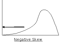
• Skewed to the left (Negative skew): The left tail is longer; more outliers on the left.

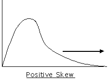
• Skewed to the right (Positive skew): The right tail is longer; more outliers on the right.

• Symmetric: Both tails are of equal length; the normal distribution is a key example.

Z-scores

Z-scores measure the relative location of a value within a dataset, indicating how many standard deviations an observation is from the mean:

• Formula: $z_i = \frac{x_i - \bar{x}}{s}$

• Interpretation: Negative z-scores are below the mean; positive are above.

• Example: For $x_2 = 54$, $\bar{x} = 44$, $s = 8$, $z_2 = 1.25$ (1.25 standard deviations above the mean).

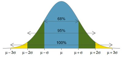
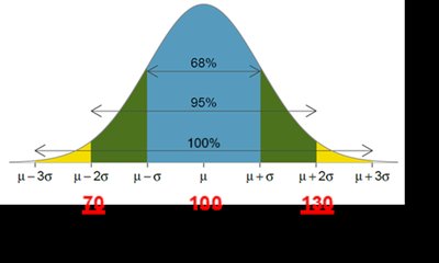
The Empirical Rule

The empirical rule applies to bell-shaped (normal) distributions, describing the percentage of data within certain standard deviations from the mean:

• Approximately 68% within 1 standard deviation

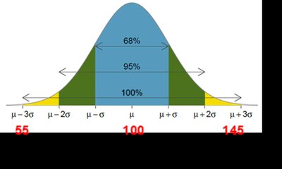
• Approximately 95% within 2 standard deviations

• Approximately 100% within 3 standard deviations

Examples Using the Empirical Rule

• IQ scores between 85 and 115 (mean 100, SD 15): 68% of people

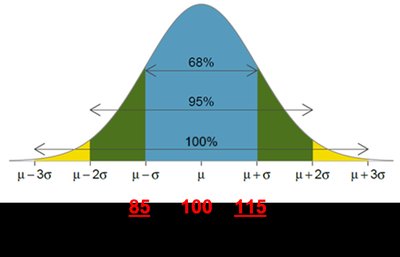
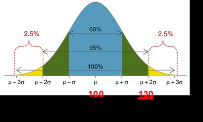
• IQ scores between 70 and 130: 95% of people

• IQ scores above 130: 2.5% of people

• 16th percentile (P16): IQ = 85

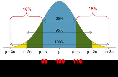
• 84th percentile (P84): IQ = 115

• Outlier detection: IQ = 160 is an outlier (z = 4, more than 3 SDs from mean)

Detecting Outliers

Outliers are extreme values that may affect statistical analysis. Two main methods for detecting outliers:

1. For bell-shaped distributions: Any value with $z < -3$ or $z > 3$ is considered an outlier.

2. For non-bell-shaped distributions: Calculate lower and upper limits:

   • Lower limit: $Q_1 - 1.5(IQR)$

   • Upper limit: $Q_3 + 1.5(IQR)$

   • Values outside these limits are outliers.

Five-Number Summaries and Boxplots

Five-Number Summary

The five-number summary consists of:

1. Minimum

2. First quartile (Q1)

3. Median (Q2)

4. Third quartile (Q3)

5. Maximum

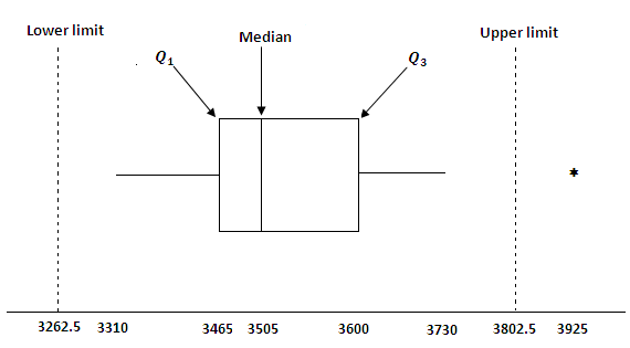
Box Plot

A box plot is a graphical summary based on the five-number summary, useful for visualizing the spread and detecting outliers:

• The box spans Q1 to Q3 (middle 50% of data).

• A line marks the median; an X may indicate the mean.

• Whiskers extend to the smallest/largest values within 1.5(IQR) of Q1/Q3.

• Outliers are plotted as individual points.

• Box plots can indicate skewness by the position of the median and the length of whiskers.

Measures of Association Between Two Variables

Covariance

Covariance measures the direction of the linear relationship between two variables X and Y:

• Formula: $s_{xy} = \frac{\sum (x_i - \bar{x})(y_i - \bar{y})}{n-1}$

• Interpretation:

  • $s_{xy} > 0$: Positive linear relationship

  • $s_{xy} < 0$: Negative linear relationship

  • $s_{xy} = 0$: No linear relationship

• Limitation: Covariance does not indicate the strength of the relationship due to dependence on units.

Correlation Coefficient

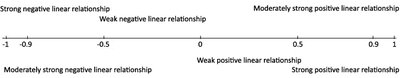
The correlation coefficient (r) measures the strength and direction of the linear relationship between two variables, standardized to be unitless:

• Formula: $r_{xy} = \frac{s_{xy}}{s_x s_y}$

• Range: $-1 \leq r_{xy} \leq 1$

• Interpretation:

  • $r_{xy} = 1$: Perfect positive linear relationship

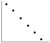
  • $r_{xy} = -1$: Perfect negative linear relationship

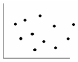
  • $r_{xy} = 0$: No linear relationship

The Weighted Mean and Grouped Data

Weighted Mean

When observations have different levels of importance, the weighted mean is used:

• Formula: $\bar{x} = \frac{\sum w_i x_i}{\sum w_i}$

• Example: Calculating the mean cost per pound for purchases with different quantities.

Grouped Data

For data presented in frequency distributions, the mean and variance can be estimated using group midpoints:

• Sample mean: $\bar{x} = \frac{\sum f_i M_i}{n}$

• Sample variance: $s^2 = \frac{\sum f_i (M_i - \bar{x})^2}{n-1}$

• Where: $M_i$ is the midpoint of the ith group, $f_i$ is the frequency, and $n$ is the total number of observations.

Summary Table: Key Measures and Their Formulas

Measure	Formula	Interpretation
Interquartile Range (IQR)	$Q_3 - Q_1$	Middle 50% spread
Variance (Sample)	$s^2 = \frac{\sum (x_i - \bar{x})^2}{n-1}$	Average squared deviation
Standard Deviation (Sample)	$s = \sqrt{s^2}$	Average deviation from mean
Coefficient of Variation	$cv = \frac{s}{\bar{x}} \times 100$	Relative variability (%)
Z-score	$z_i = \frac{x_i - \bar{x}}{s}$	Relative position in SD units
Covariance	$s_{xy} = \frac{\sum (x_i - \bar{x})(y_i - \bar{y})}{n-1}$	Direction of linear relationship
Correlation Coefficient	$r_{xy} = \frac{s_{xy}}{s_x s_y}$	Strength and direction of linear relationship
Weighted Mean	$\bar{x} = \frac{\sum w_i x_i}{\sum w_i}$	Mean with weights
Grouped Data Mean	$\bar{x} = \frac{\sum f_i M_i}{n}$	Mean for grouped data