Summarizing Data in Tables and Graphs: Introductory Statistics Study Guide

Summarizing Data in Tables and Graphs

Organizing Qualitative Data

Frequency Distributions

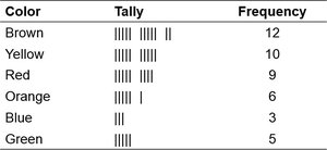
Qualitative data, such as survey responses or categorical variables, must be organized to facilitate analysis. A frequency distribution lists each category and the number of occurrences for each category.

• Raw data refers to unorganized data.

• Frequency table is a common method for organizing qualitative data.

• Each row represents a category, with columns for tally marks and frequency counts.

Example: Frequency distribution of M&M colors in a sample.

Relative Frequency Distributions

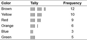
The relative frequency is the proportion or percentage of observations within a category. It is calculated as:

• $\text{Relative Frequency} = \frac{\text{Frequency of Category}}{\text{Total Frequency}}$

• Relative frequencies allow comparison between categories, especially when sample sizes differ.

Example: Relative frequency distribution for M&M colors.

Constructing Bar Graphs

Bar Graphs for Qualitative Data

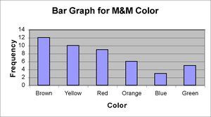
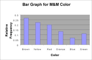
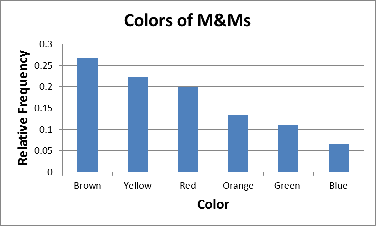
A bar graph visually represents the frequency or relative frequency of each category. Categories are labeled on one axis, and frequencies on the other. Bars are of equal width and do not touch.

• Bar graphs can display either frequency or relative frequency.

• Useful for comparing categorical data.

Example: Frequency bar graph for M&M colors.

Example: Relative frequency bar graph for M&M colors.

Pareto Charts

A Pareto chart is a bar graph where bars are ordered from highest to lowest frequency or relative frequency. This helps highlight the most common categories.

• Useful for identifying the most significant categories in a dataset.

Side-by-Side and Horizontal Bar Graphs

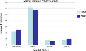
Side-by-side bar graphs compare two or more groups across categories, often using relative frequencies for fair comparison. Horizontal bar graphs are preferable when category names are lengthy.

Example: Comparison of marital status in 1990 vs. 2006.

Pie Charts

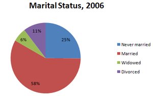
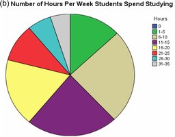
A pie chart divides a circle into sectors, each representing a category. The area of each sector is proportional to the frequency or relative frequency of the category.

• Useful for showing parts of a whole.

Example: Pie chart of marital status in 2006.

Organizing Quantitative Data

Discrete Data

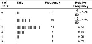
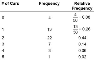
Discrete quantitative data can be organized in frequency and relative frequency tables. If there are few values, each value forms a category.

• Example: Number of cars per household.

Histograms for Discrete Data

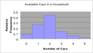
A histogram is constructed by drawing rectangles for each class of data. The height represents frequency or relative frequency, and rectangles touch each other.

Example: Frequency histogram for number of cars per household.

Example: Relative frequency histogram for number of cars per household.

Continuous Data

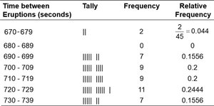
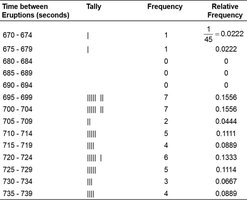
Continuous data are grouped into classes (intervals). The lower class limit is the smallest value in a class, and the upper class limit is the largest. Class width is the difference between consecutive lower class limits.

• Classes are chosen to best summarize the data, typically between 5 and 20 classes.

• Example: Time between eruptions at Old Faithful Geyser.

Determining Number of Classes

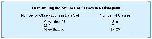
The number of classes in a histogram depends on the size of the data set:

Number of Observations	Number of Classes
Fewer than 25	5-6
25-50	7-14
More than 50	15-20

Stem-and-Leaf Plots

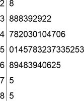
A stem-and-leaf plot displays data by splitting each value into a "stem" (all but the last digit) and a "leaf" (the last digit). This plot preserves the original data values.

• Stems are listed vertically, leaves are listed horizontally.

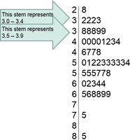
• Split stems can be used for bunched data.

Dot Plots

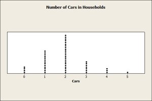
A dot plot places each observation horizontally in increasing order, with a dot above each value for every occurrence.

• Useful for small data sets and visualizing clusters or gaps.

Identifying the Shape of a Distribution

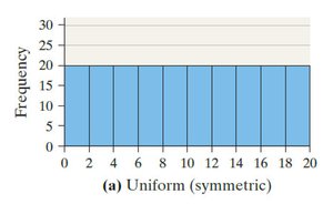
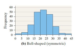
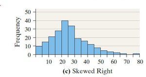
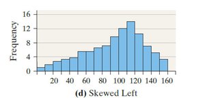
The shape of a distribution can be classified as:

• Uniform: Frequencies are evenly spread.

• Bell-shaped: Highest frequency in the middle, tails off at both ends.

• Skewed right: Tail on the right is longer.

• Skewed left: Tail on the left is longer.

Time Series Graphs

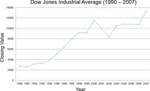
Time series data are measured at different points in time. A time-series plot shows time on the horizontal axis and the variable's value on the vertical axis, connecting points with line segments.

Graphical Misrepresentations of Data

Misleading or Deceptive Graphs

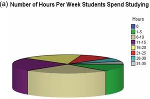
Graphs can be misleading if they distort the data, exaggerate differences, or use inappropriate scales. Guidelines for constructing good graphics include:

• Title and label axes clearly, including units and data sources.

• Avoid distortion and minimize white space.

• Avoid clutter and unnecessary backgrounds.

• Do not use three-dimensional effects that distract or mislead.

• Do not use more than one design in the same graphic.

• Always include data and scales.

Example: Misleading pie chart exaggerating student study hours.

Example: Proper pie chart for student study hours.

Summary Table: Types of Graphical Displays

Type	Purpose	Data Type
Frequency Table	Organize counts by category	Qualitative/Discrete Quantitative
Bar Graph	Visualize frequencies/relative frequencies	Qualitative
Pareto Chart	Highlight most frequent categories	Qualitative
Pie Chart	Show proportions of a whole	Qualitative
Histogram	Visualize distribution	Quantitative
Stem-and-Leaf Plot	Preserve raw data, visualize shape	Quantitative
Dot Plot	Visualize individual values	Quantitative
Time Series Plot	Show trends over time	Quantitative (time series)

Additional info: These notes expand on brief points from the original slides, providing definitions, examples, and academic context for each graphical method.