Summarizing Important Features of a Numerical Distribution

Describing Data with Tables and Graphs

Summarizing Important Features of a Numerical Distribution

When analyzing a numerical distribution, it is essential to describe its shape, center, and spread (variability), as well as to identify any outliers. These characteristics help us understand the underlying patterns and tendencies in the data.

Shape of a Distribution

The shape of a distribution refers to the general form of its graph. Key aspects include symmetry, skewness, and the number of peaks (modes).

• Symmetric Distribution: The left and right sides of the graph are mirror images. The most common example is the bell-shaped curve (normal distribution).

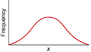
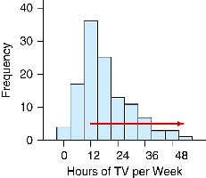
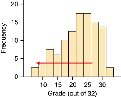
• Skewed Distribution: The graph is not symmetric. It can be skewed to the right (longer tail on the right) or to the left (longer tail on the left).

• Right Skewed: Most data are concentrated on the left, with a tail extending to the right.

• Left Skewed: Most data are concentrated on the right, with a tail extending to the left.

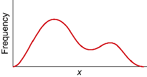
• Number of Mounds (Modes): Distributions can be unimodal (one peak), bimodal (two peaks), or multimodal (more than two peaks).

• Unimodal: A single peak.

• Bimodal: Two distinct peaks.

Outliers and Extreme Values

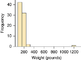
Outliers are data points that are significantly different from the rest of the data. They can affect the interpretation of the distribution's center and spread.

• Outliers are often visible as isolated bars or points far from the main cluster of data in a histogram.

Center of a Distribution

The center of a distribution is a typical value around which the data are distributed. Common measures of center include the mean, median, and mode.

• Mean: The arithmetic average of all data values.

• Median: The middle value when data are ordered from least to greatest.

• Mode: The most frequently occurring value.

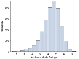
Example: The histogram below shows audience movie ratings. The typical rating (center) is around 7.

Spread (Variability) of a Distribution

The spread or variability describes how much the data values differ from each other. Common measures include the range, interquartile range (IQR), and standard deviation.

• Range: The difference between the maximum and minimum values.

• Interquartile Range (IQR): The range of the middle 50% of the data.

• Standard Deviation: A measure of the average distance of data points from the mean.

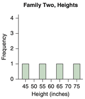
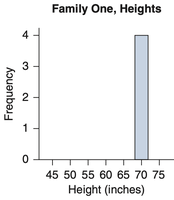
Distributions with similar values have a narrow spread, while those with diverse values have a wider spread.

Describing a Numerical Distribution

To fully describe a numerical distribution, always mention:

1. Shape: Is it symmetric, skewed left, or skewed right? How many modes?

2. Center: What is a typical value?

3. Variability: How spread out are the values? Are there any outliers?

Examples and Applications

• GPA of college students: Often slightly left-skewed, as more students have higher GPAs.

• SAT scores: Typically symmetric and bell-shaped (normal distribution).

• Last digit of Social Security numbers: Uniform distribution (all digits equally likely).

• Income of USA residents: Strongly right-skewed due to a small number of very high incomes.

Summary Table: Key Features of a Numerical Distribution

Feature	Description	Example
Shape	Symmetric, skewed left, skewed right, unimodal, bimodal	Bell curve, right-skewed income
Center	Mean, median, mode	Average movie rating
Spread	Range, IQR, standard deviation	Height variability in families
Outliers	Unusually high or low values	Extreme weight in a sample

Additional info: Measures of center and spread are covered in more detail in later sections, including how to calculate mean, median, and standard deviation.