Summarizing Numerical Distributions: Shape, Center, and Spread

Section 2.2 Summarizing Important Features of a Numerical Distribution

Shape, Center, and Spread

When analyzing numerical data distributions, it is essential to describe three main features: shape, center, and spread. These characteristics help us understand the overall pattern, typical values, and variability within the data.

• Shape: Refers to the general form of the distribution, including symmetry, skewness, and the number of modes (mounds).

• Center: Represents the typical value around which data points cluster.

• Spread: Indicates the variability or dispersion of the data values.

Examining a Distribution

To thoroughly describe a distribution, pay attention to:

• The shape of the distribution (symmetric, skewed, number of modes).

• The center or typical value.

• The spread or variability.

Shape of a Distribution

Shape is a fundamental aspect of describing a distribution. The three basic characteristics to consider are:

• Is the distribution symmetric or skewed?

• How many mounds (peaks) appear?

• Are there any outliers (extremely large or small values)?

Symmetric Distributions

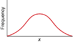
A symmetric distribution has left and right sides that are roughly mirror images of each other. The most common example is the bell-shaped (normal) distribution.

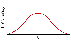
Skewed Distributions

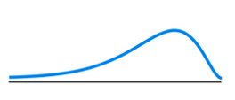
A skewed distribution is not symmetric. If the tail extends to the right, it is right-skewed; if the tail extends to the left, it is left-skewed.

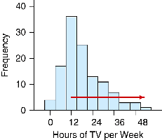
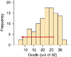
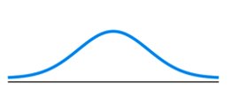
Distribution Shapes: Bell, Right Skewed, Left Skewed

Common shapes include bell-shaped (normal), right-skewed, and left-skewed distributions.

Shape: Mounds (Modes)

Distributions can be classified by the number of mounds (modes):

• Unimodal: One main mound.

• Bimodal: Two main mounds.

• Multimodal: More than two mounds.

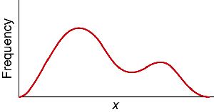
Note: Bimodal and multimodal distributions may indicate the presence of different groups within the data. For example, heights of men and women or sales at different times of day.

Shape: Examples

Expected shapes for common data sets:

• GPA of college students: Skewed left

• SAT scores: Symmetric (Unimodal)

• Last digit of Social Security numbers: Symmetric (Uniform)

• Income of USA residents: Skewed right

Outliers

Outliers are extremely large or small values that do not fit the pattern of the rest of the data. They are not precisely defined and may be subject to opinion. Outliers can result from data entry errors or may represent genuinely interesting observations.

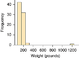
• Report outliers when observed.

• Consider their potential as sources of error or as significant data points.

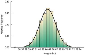
Distribution Shape Example

Example: The distribution of heights of female students at a college is bell-shaped.

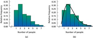
Distribution Shape Example: Household Size

Example: The distribution of household size in the U.S. is right-skewed.

Center of a Distribution

The center of a distribution is the typical data value. It is often estimated by the mean or median, depending on the shape and presence of outliers.

• For symmetric distributions, the mean is a good measure of center.

• For skewed distributions, the median is often preferred.

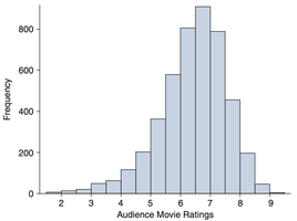
Example: Audience movie ratings for English-language films have a center around 6.5 points.

Center Example: Soccer Goals

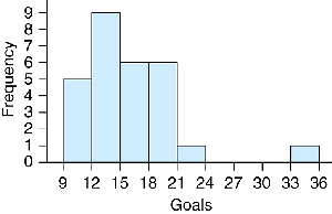
Example: Histograms for Division III first-year women and men soccer players in 2012 show:

• Women: Typical score is 16 goals.

• Men: Typical score is 13 goals.

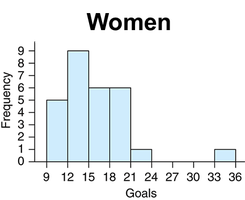
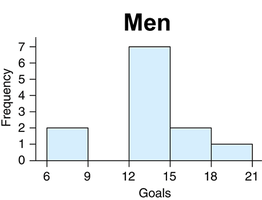
This suggests that the typical male soccer player scores fewer goals than the typical female player.

Why Not the Mode?

The mode is the most frequently occurring value. For numerical data, it is generally not recommended to use the mode, especially when reading from a histogram, because:

• Histograms can obscure the location of the mode due to bin width.

• There can be multiple modes in a data set.

• The mode can change with minor data adjustments.

Variability (Spread)

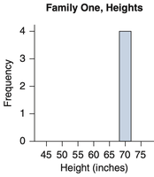
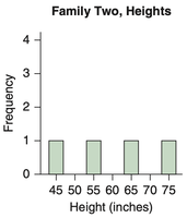
Variability refers to the horizontal spread of the data in a histogram or dotplot. It indicates how similar or different the data values are.

• If all data values are similar: The graph is narrow.

• If data values are different: The graph is wider.

Variability Example

Example: A narrow graph indicates low variability, while a wide graph indicates high variability.

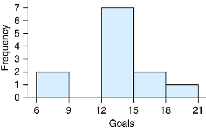
Describing Numerical Distributions: Summary

Always describe a numerical distribution using these three components:

• Shape: Symmetric, skewed left/right, number of modes

• Center: Typical value (mean or median)

• Variability: Horizontal spread (range, standard deviation, interquartile range)

These features provide a comprehensive summary of the data and are foundational for further statistical analysis.