The Central Limit Theorem and Sampling Distributions

The Central Limit Theorem and Sampling Distributions

Introduction to Sampling Distributions

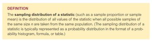
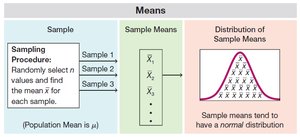
The concept of a sampling distribution is fundamental in statistics, especially when analyzing the behavior of sample means. A sampling distribution describes the distribution of a statistic (such as the sample mean or sample proportion) when all possible samples of a given size are drawn from the same population. Understanding sampling distributions is essential for making inferences about population parameters based on sample data.

Simulation of Sampling Distributions

Statistical software, such as StatCrunch, can be used to simulate sampling distributions for various statistics and populations. This allows for the exploration of concepts such as the Central Limit Theorem and the behavior of sample means.

Sampling from a Uniform Distribution

Consider a random variable X with a uniform distribution, X ~ U(0, 50). The mean and standard deviation of the original population are important reference points for understanding the sampling distribution of sample means.

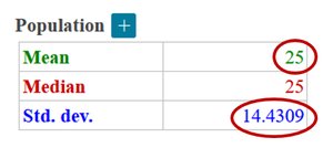
• Mean: 25

• Median: 25

• Standard deviation: 14.4309

When calculating the mean of thousands of samples for different sample sizes (n = 4, 16, 100), observe the following:

• Shape: As n increases, the sampling distribution of means becomes more normal in shape.

• Center: The mean of the sampling distribution remains close to the population mean.

• Spread: The standard deviation of the sampling distribution decreases as n increases.

Visualizing the Central Limit Theorem

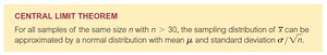
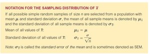
The Central Limit Theorem (CLT) states that for all samples of the same size n with n > 30, the sampling distribution of the sample mean can be approximated by a normal distribution, regardless of the shape of the original population distribution. The mean of the sampling distribution is equal to the population mean, and the standard deviation is equal to the population standard deviation divided by the square root of n.

• Formula for the mean of sample means: $\mu_{\bar{x}} = \mu$

• Formula for the standard deviation of sample means: $\sigma_{\bar{x}} = \frac{\sigma}{\sqrt{n}}$

Comparison of Sampling Distributions

The shape of the sampling distribution of the sample mean depends on the sample size and the shape of the original population distribution. As sample size increases, the sampling distribution becomes more normal, even if the original population is not normal.

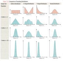
Population Shape	Sample Size n = 2	Sample Size n = 5	Sample Size n = 30
Uniform	Wide, flat	More peaked	Normal-like
Bimodal	Two peaks	Peaks merge	Normal-like
Skewed	Skewed	Less skewed	Normal-like
Normal	Normal	Normal	Normal

Example: If the original population is skewed, the sampling distribution of the mean will become more normal as n increases.

Applications of the Central Limit Theorem

The Central Limit Theorem is used to calculate probabilities related to sample means. For example, if body temperatures are normally distributed with mean 98.2°F and standard deviation 0.6°F, the probability that a randomly selected person has a temperature above 99°F can be calculated using the normal distribution. For a group of 16 people, the sampling distribution of the mean is used, with standard deviation $\frac{0.6}{\sqrt{16}} = 0.15$.

• Formula for z-score of sample mean: $z = \frac{x - \mu}{\sigma / \sqrt{n}}$

• Application: Use the z-score to find probabilities and percentiles for sample means.

Example: For Tylenol weights, if X ~ N(605.1 mg, 5.96 mg), the probability of observing an average weight of 600 mg in a sample of 20 pills can be calculated using the sampling distribution of the mean.

Additional info: The probability of seeing a statistic at least as extreme as x is called a p-value, which is discussed further in hypothesis testing (Chapter 8).