The Normal Distribution: Concepts, Calculations, and Applications

The Normal Distribution

General Properties and Importance

The normal distribution is a fundamental concept in statistics, characterized by its symmetric, bell-shaped curve. It is widely used because many real-world variables, especially those influenced by numerous random factors, tend to follow this distribution. The standard normal distribution is a special case with a mean of 0 and a standard deviation of 1, serving as a mathematical tool for analyzing data.

• Areas under the curve represent relative frequencies, percentages (as decimals), and probabilities.

• Variables influenced by many independent random factors (e.g., human height) are often approximately normally distributed.

• The normal distribution arises naturally when many random effects are combined, as illustrated by the Galton Machine (Quincunx).

Example: The heights of female college students are normally distributed with a mean (μ) of 64.4 inches and a standard deviation (σ) of 2.4 inches.

Standardization: z-Scores

To use the standard normal table, observed values (x) must be converted to z-scores, which measure how many standard deviations a value is from the mean. This process is called standardization.

• Formula:

$z = \frac{x - \mu}{\sigma}$

• Where x is the observed value, μ is the mean, and σ is the standard deviation.

• Once standardized, z-scores can be used to find probabilities and percentages using the standard normal table.

Calculating Probabilities and Percentages

Percentages and probabilities for values less than or greater than a given x are found by calculating the z-score and using the normal table or calculator functions.

• "Less than" corresponds to the area to the left of the z-score.

• "Greater than" corresponds to the area to the right of the z-score.

• To find the percentage between two values, subtract the area to the left of the lower value from the area to the left of the higher value.

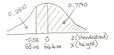
Example: To find the percentage of female college students between 63 and 68 inches tall:

• Standardize both values:

$z_{63} = \frac{63 - 64.4}{2.4} = -0.58$ $z_{68} = \frac{68 - 64.4}{2.4} = 1.50$

• Find areas using the table: Area to left of -0.58 is 0.2810; area to left of 1.50 is 0.9332.

• Percentage between: $0.9332 - 0.2810 = 0.6522 = 65.22\%$

Calculator Methods

Modern calculators can compute areas under the normal curve for any mean and standard deviation using the normalcdf function:

• normalcdf(a, b, μ, σ) gives the area between values a and b.

• For example, normalcdf(63, 68, 64.4, 2.4) yields the percentage between 63 and 68 inches.

Inverse Normal Calculations: Finding x from Percentages

Sometimes, we are given a percentage or probability and need to find the corresponding x-value. This is called the inverse normal procedure.

• First, find the z-score corresponding to the desired area using the table.

• Then, "destandardize" using the formula:

$x = \mu + z \cdot \sigma$

• Where z is the z-score for the desired percentile.

• Calculator shortcut: Invnorm(P, μ, σ) gives the x-value for percentile P.

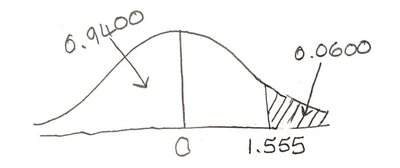
Example: To find the height separating the tallest 6% from the rest:

• Area to left is 0.94; z ≈ 1.555.

• $x = 64.4 + 1.555 \times 2.4 = 68.13$ inches.

Summary of Procedures

• To find probabilities given x-values: Standardize (find z), then use the table or calculator.

• To find x-values given probabilities: Find z from the table or calculator, then destandardize.

Table-based method:

• Standardize → Table (outside-to-in)

• Destandardize → Table (inside-to-out)

Calculator-based method:

• normalcdf(a, b, μ, σ) for areas between values

• Invnorm(P, μ, σ) for x-values at given percentiles

Normal Probability Plots

Researchers use normal probability plots to assess whether sample data is approximately normally distributed. While constructing these plots is not required in this course, they are useful for verifying the appropriateness of normal distribution methods.

• Histograms can visually suggest normality, but formal tests and plots provide more objective evidence.

• Normal probability plots compare sample data to expected values under a normal distribution.

Additional info: Section 6.4 in textbooks often covers normal probability plots, but students are not required to construct them for this course.