The Normal Distribution, Sampling Distribution, and the Central Limit Theorem: Study Guide

The Normal Distribution, Sampling Distribution, and the Central Limit Theorem

Normal Distribution

The normal distribution is a fundamental concept in statistics, describing a continuous probability distribution that is symmetric about its mean. It is characterized by its bell-shaped curve and is used to model many natural phenomena.

• Key Properties:

  • Mean, median, and mode are all equal.

  • Symmetrical about the mean.

  • Defined by two parameters: mean (μ) and standard deviation (σ).

  • The total area under the curve is 1.

• Empirical Rule:

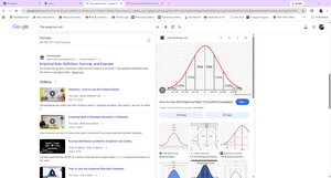
  • Approximately 68% of data falls within 1 standard deviation of the mean.

  • Approximately 95% within 2 standard deviations.

  • Approximately 99.7% within 3 standard deviations.

• Formula: $f(x) = \frac{1}{\sigma \sqrt{2\pi}} e^{-\frac{1}{2} \left( \frac{x-\mu}{\sigma} \right)^2}$

Distribution of Individual Values

Individual values in a population are distributed according to the population's distribution, which may be normal or non-normal. When the population is normal, individual values follow the normal curve.

Distribution of Sample Means

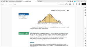
The distribution of sample means refers to the probability distribution of means calculated from all possible samples of a given size drawn from a population. This distribution is central to inferential statistics.

• Sample means tend to cluster around the population mean.

• The spread (standard deviation) of sample means is less than that of individual values.

Properties of the Distribution of Sample Means

The distribution of sample means has several important properties:

• The mean of the sample means equals the population mean (μ).

• The standard deviation of the sample means (standard error) is $\frac{\sigma}{\sqrt{n}}$.

• As sample size increases, the distribution becomes more concentrated around the mean.

The Central Limit Theorem (CLT)

The Central Limit Theorem is a foundational principle in statistics. It states that, regardless of the population's distribution, the distribution of sample means approaches a normal distribution as the sample size increases (typically n ≥ 30).

• If the original population is normal: The sampling distribution of the mean is normal for any sample size.

• If the original population is not normal: The sampling distribution of the mean becomes approximately normal as n increases (n ≥ 30).

Notation and Formulas

• Mean of sample means: $\mu_{\bar{x}} = \mu$

• Standard error of the mean: $\sigma_{\bar{x}} = \frac{\sigma}{\sqrt{n}}$

• Z-score for sample mean: $z = \frac{\bar{x} - \mu}{\sigma / \sqrt{n}}$

Solving Problems Using the CLT

The CLT allows us to use the normal distribution to solve problems about sample means, using the standard error in place of the population standard deviation.

• Convert sample mean to a z-score using the formula above.

• Use z-tables to find probabilities associated with sample means.

Worked Examples

Example: Hours of Television Watched by Children

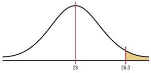
Given: Mean = 25 hours, Standard deviation = 3 hours, Sample size = 20. Find the probability that the sample mean exceeds 26.3 hours.

• Since the variable is normally distributed, use the CLT formula for z-score.

• Calculate standard error: $\sigma_{\bar{x}} = \frac{3}{\sqrt{20}}$

• Find z-score: $z = \frac{26.3 - 25}{3 / \sqrt{20}}$

• Use z-table to find probability.

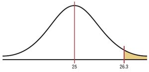
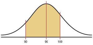
Example: Age of Boats

Given: Mean = 96 months, Standard deviation = 16 months, Sample size = 36. Find the probability that the sample mean is between 90 and 100 months.

• Sample size ≥ 30, so normality assumption is not necessary.

• Calculate standard error: $\sigma_{\bar{x}} = \frac{16}{\sqrt{36}} = 2.67$

• Find z-scores for 90 and 100 months.

• Use z-table to find probability between these values.

Example: Pork Consumption (Individual Value)

Given: Mean = 218.4 pounds, Standard deviation = 25 pounds. Find the probability that a randomly selected person consumes less than 224 pounds per year.

• Calculate z-score: $z = \frac{224 - 218.4}{25}$

• Use z-table to find probability.

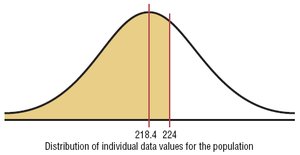
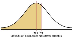
Example: Pork Consumption (Sample Mean)

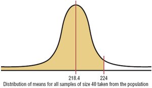
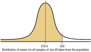
Given: Mean = 218.4 pounds, Standard deviation = 25 pounds, Sample size = 40. Find the probability that the sample mean is less than 224 pounds per year.

• Calculate standard error: $\sigma_{\bar{x}} = \frac{25}{\sqrt{40}}$

• Find z-score: $z = \frac{224 - 218.4}{25 / \sqrt{40}}$

• Use z-table to find probability.

Summary Table: Properties of Normal and Sampling Distributions

Distribution	Mean	Standard Deviation	Shape
Individual Values	μ	σ	Depends on population
Sample Means	μ	σ/√n	Normal if n ≥ 30 or population is normal

Additional info: Academic context and formulas were expanded for clarity and completeness. Duplicate images were included only when they directly reinforce the explanation of the adjacent paragraph.