 Back
The Normal Probability Distribution: Concepts, Properties, and Applications
Study Guide - Smart Notes
 Tailored notes based on your materials, expanded with key definitions, examples, and context.
The Normal Probability Distribution
Introduction to Continuous Probability Distributions
The normal probability distribution is a fundamental concept in statistics, describing how data values are distributed for many natural phenomena. It is a type of continuous probability distribution, meaning the random variable can take any value within a given range. Understanding the properties and applications of the normal distribution is essential for statistical inference and data analysis.
Probability Density Functions and Uniform Distribution
Probability Density Function (PDF)
A probability density function (PDF) is an equation used to compute probabilities for continuous random variables. It must satisfy two properties:
The total area under the graph of the equation over all possible values of the random variable must equal 1.
The height of the graph must be greater than or equal to 0 for all possible values.
For continuous random variables, probabilities are assigned to intervals, not individual values, since the probability of any single value is zero.
Uniform Probability Distribution Example
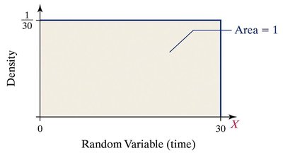
The uniform distribution is a simple continuous distribution where all intervals of equal length are equally likely. For example, if a friend can be late between 0 and 30 minutes, the probability density is constant across this interval.
The height of the rectangle is , and the area under the curve is 1.
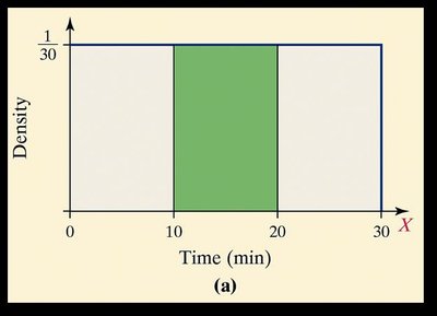
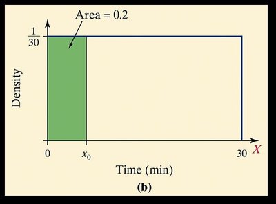
To find the probability for an interval, multiply the height by the width of the interval.
Calculating Probabilities Using Area
Probability your friend is between 10 and 20 minutes late: Area = .
Probability your friend arrives within the next 6 minutes: Area = .
Discrete vs. Continuous Variables
Classification of Variables
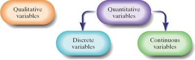
Variables in statistics are classified as:
Qualitative variables: Describe categories or qualities.
Quantitative variables: Describe numerical values and can be further classified as:
Discrete variables: Finite or countable values (e.g., 0, 1, 2, 3).
Continuous variables: Infinite values, measurable to any desired accuracy.
Continuous Probability Distributions
Key Properties
Continuous probability distributions are represented by curves. Probabilities are found by calculating the area under the curve for a given interval. The total area under the curve is always 1.
Probability of a single value is 0.
Probabilities are assigned to intervals.
The Normal Distribution
Definition and Properties
The normal distribution is the most commonly used continuous distribution. It is characterized by its bell-shaped, symmetric curve. The curve theoretically extends infinitely in both directions and the total area under the curve is 1.
Mean, median, and mode are equal.
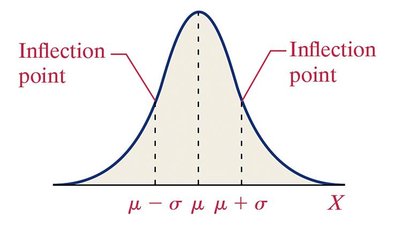
Inflection points occur at and .
Area to the left and right of the mean is equal (0.5 each).
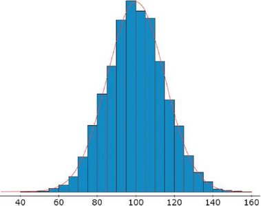
Visualizing Normal Distribution
Histograms of real data often approximate the normal curve, especially for large samples.
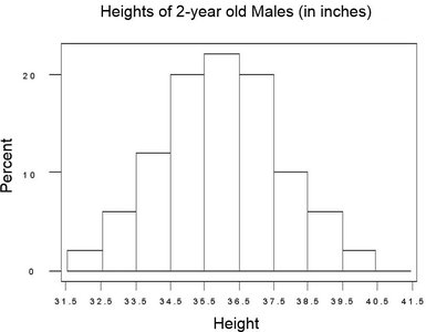
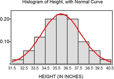
Inflection Points and Empirical Rule
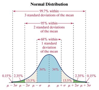
The points and are inflection points where the curvature changes. The Empirical Rule states:
68% of data within 1 standard deviation of the mean
95% within 2 standard deviations
99.7% within 3 standard deviations
Area Under the Normal Curve
Interpretation of Area
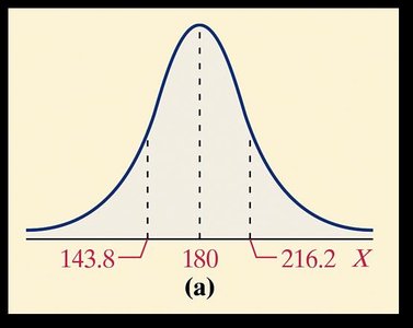
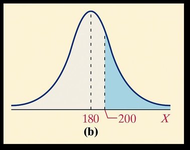
The area under the normal curve for an interval represents:
The proportion of the population with the characteristic described by the interval
The probability that a randomly selected individual has the characteristic
Standardizing Normal Random Variables
Z-Scores and the Standard Normal Distribution
A z-score is a standardized value that indicates how many standard deviations a value is from the mean:
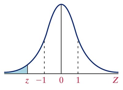
The standard normal distribution has mean 0 and standard deviation 1.
Using the Standard Normal Table
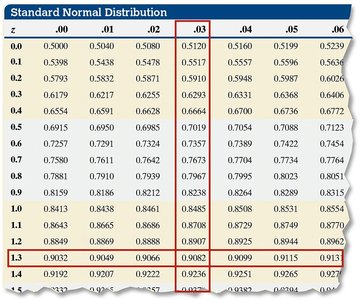
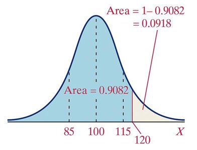
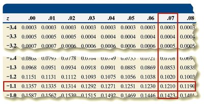
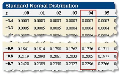
The standard normal table provides areas to the left of a given z-score. For example, for , the area is 0.9082.
Finding Probabilities with the Standard Normal Table
Step-by-Step Procedure
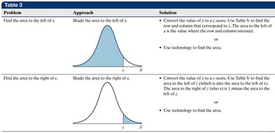
Draw the normal curve and shade the area of interest.
Convert x-values to z-scores.
Look up the corresponding areas in the standard normal table.
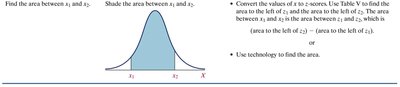
Manipulate the areas as needed (e.g., use complement rule or subtract areas for intervals).
Examples and Applications
Example: Pediatric Heights
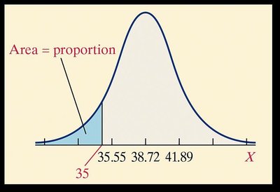
Heights of three-year-old females are normally distributed with mean 38.72 inches and standard deviation 3.17 inches. To find the proportion less than 35 inches:
Convert 35 to z-score:
Area to the left of is 0.1210
Example: Probability Between Two Values
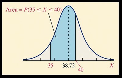
Probability a randomly selected three-year-old female is between 35 and 40 inches tall:
Convert both values to z-scores: ,
Area between and is
Percentiles and "Working Backwards"
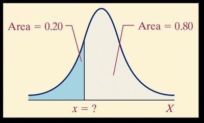
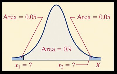
To find the value corresponding to a given percentile:
Draw the normal curve and identify the area.
Find the z-score for the area using the standard normal table.
Convert the z-score to the original variable:
Notation and Special Z-Scores
zα Notation
The notation refers to the z-score such that the area to the right of is . For example, is the z-score with 0.10 area to its right.
Summary Table: Properties of the Normal Distribution
Property | Description |
|---|---|
Shape | Bell-shaped, symmetric |
Mean, Median, Mode | All equal |
Inflection Points | At and |
Total Area | 1 |
Empirical Rule | 68% within 1 SD, 95% within 2 SD, 99.7% within 3 SD |
Standardization |
Additional info:
All equations are provided in LaTeX format for clarity and academic rigor.
Examples are expanded for self-contained understanding.
Images are included only when directly relevant to the explanation.
