The Normal Probability Distribution: Properties, Applications, and Approximations

The Normal Probability Distribution

Uniform Probability Distribution

The uniform probability distribution is a type of continuous probability distribution where all outcomes are equally likely within a certain interval. The probability density function (pdf) for a uniform distribution is constant between two values and zero elsewhere.

• Key Properties:

  • The total area under the pdf over all possible values equals 1.

  • The height of the pdf is always greater than or equal to 0.

  • For a uniform distribution on the interval [a, b], the pdf is $f(x) = \frac{1}{b-a}$ for $a \leq x \leq b$.

• Example: If the random variable X represents time between 0 and 60 minutes, the pdf is $f(x) = \frac{1}{60}$ for $0 \leq x \leq 60$.

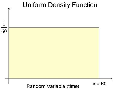
The area under the curve between two points represents the probability that the random variable falls within that interval. For example, $P(15 < X < 30) = \frac{15}{60} = 0.25$.

Normal Probability Distribution

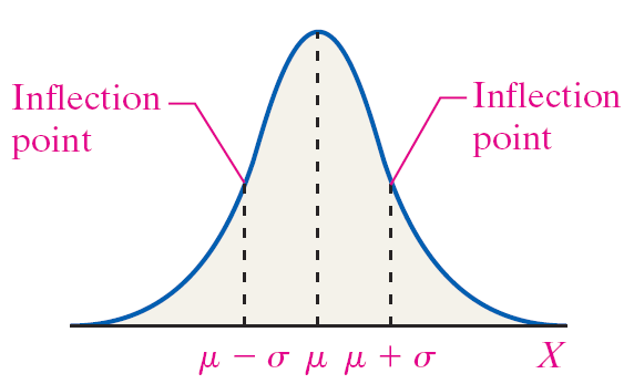
The normal distribution is a continuous probability distribution that is symmetric and bell-shaped. It is one of the most important distributions in statistics due to its natural occurrence in many real-world phenomena.

• Key Properties:

  • Symmetric about its mean $\mu$.

  • Mean = median = mode; the highest point occurs at $x = \mu$.

  • Inflection points at $\mu - \sigma$ and $\mu + \sigma$, where $\sigma$ is the standard deviation.

  • Total area under the curve is 1.

  • Area to the left and right of the mean is 0.5 each.

  • As $x$ approaches $\pm\infty$, the curve approaches but never touches the horizontal axis.

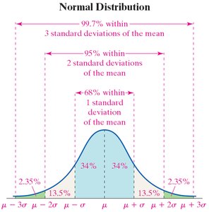
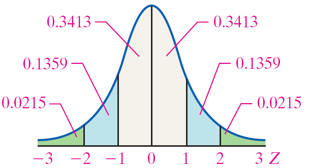
  • Empirical Rule:

    • Approximately 68% of data within $\mu \pm \sigma$

    • Approximately 95% within $\mu \pm 2\sigma$

    • Approximately 99.7% within $\mu \pm 3\sigma$

Graphing and Interpreting Normal Curves

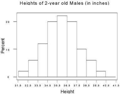
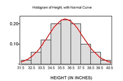
Relative frequency histograms that are symmetric and bell-shaped approximate the normal curve. Many real-world variables, such as heights or test scores, are approximately normally distributed.

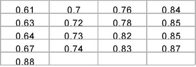
• Example: The distribution of heights of 2-year-old males can be visualized with a histogram and compared to a normal curve.

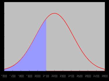
Area Under the Normal Curve

The area under the normal curve for an interval represents the probability or proportion of observations within that interval. For a normally distributed variable $X$ with mean $\mu$ and standard deviation $\sigma$:

• The area under the curve between $a$ and $b$ is $P(a < X < b)$.

• This area can be interpreted as the probability that a randomly selected value falls in that interval, or the proportion of the population with that characteristic.

Applications of the Normal Distribution

Standardizing a Normal Random Variable (Z-scores)

To compare values from different normal distributions or to use standard normal tables, we convert values to z-scores:

• The z-score for a value $x$ is $z = \frac{x - \mu}{\sigma}$.

• The standard normal distribution has $\mu = 0$ and $\sigma = 1$.

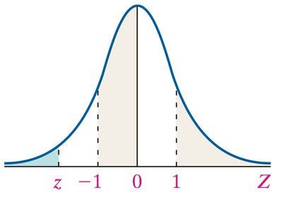
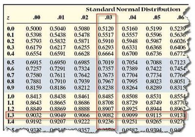
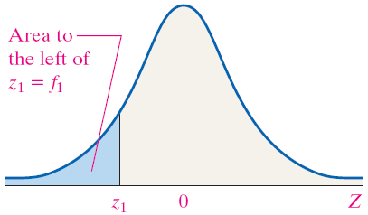
Using the Standard Normal Table

The standard normal table (Table V) gives the area to the left of a specified z-score. This area represents the probability that a standard normal variable is less than or equal to $z$.

• Example: For $z = 1.33$, the area to the left is 0.9082, meaning 90.82% of values are below this z-score.

Finding Areas and Probabilities

• To find the area to the right of a z-score, subtract the area to the left from 1.

• To find the area between two z-scores, subtract the area to the left of the lower z from the area to the left of the higher z.

Finding Values from Areas (Percentiles)

To find the value $x$ corresponding to a given percentile or area:

1. Find the z-score corresponding to the area using the standard normal table.

2. Convert back to the original scale: $x = \mu + z\sigma$.

• Example: For the 85th percentile on a test with $\mu = 1049$ and $\sigma = 189$, $z = 1.04$, so $x = 1049 + 1.04 \times 189 = 1246$.

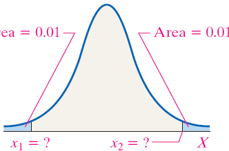
Finding Central Intervals

To find the values that bound the middle percentage (e.g., middle 90%) of a normal distribution:

• Find the z-scores that leave the desired area in the center (e.g., 0.05 in each tail for 90%).

• Convert these z-scores to x-values using $x = \mu + z\sigma$.

Assessing Normality

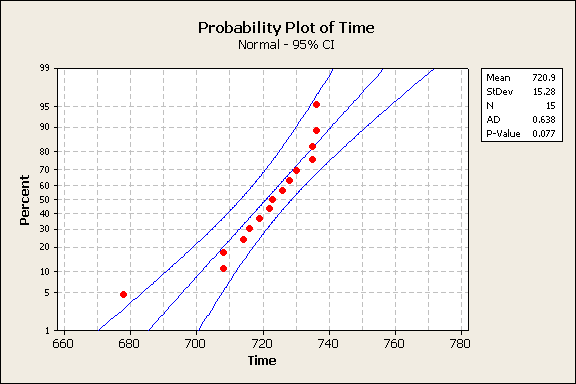
Normal Probability Plots

A normal probability plot is used to assess whether a data set is approximately normally distributed. If the data are normal, the plot will be approximately linear.

1. Order the data from smallest to largest.

2. Compute the expected proportion for each data point: $f_i = \frac{i - 0.375}{n + 0.25}$, where $i$ is the rank and $n$ is the sample size.

3. Find the z-score corresponding to each $f_i$.

4. Plot the observed values (x-axis) against the expected z-scores (y-axis).

• If the points fall roughly along a straight line, the data are likely normal.

The Normal Approximation to the Binomial Distribution

Criteria for Binomial Experiments

• Fixed number of independent trials ($n$).

• Each trial has two outcomes: success or failure.

• Probability of success ($p$) is constant for each trial.

When to Use the Normal Approximation

If $np(1-p) \geq 10$, the binomial distribution can be approximated by a normal distribution with:

• Mean: $\mu_X = np$

• Standard deviation: $\sigma_X = \sqrt{np(1-p)}$

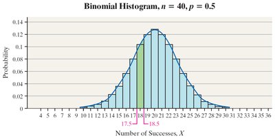
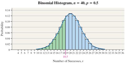
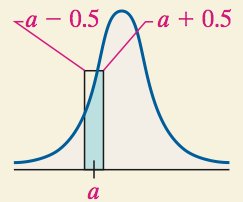
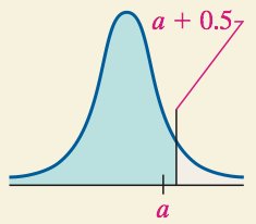
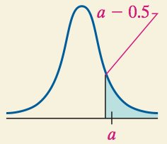
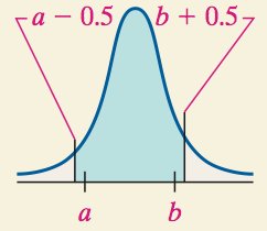
Continuity Correction

When using the normal approximation for discrete binomial probabilities, apply a continuity correction:

• For $P(X = a)$, use $P(a - 0.5 < X < a + 0.5)$

• For $P(X \leq a)$, use $P(X < a + 0.5)$

• For $P(X \geq a)$, use $P(X > a - 0.5)$

• For $P(a \leq X \leq b)$, use $P(a - 0.5 < X < b + 0.5)$

Example: Normal Approximation to the Binomial

• Suppose 35% of households have three or more cars. In a sample of 400 households, $\mu = 140$, $\sigma = 9.54$.

• To find $P(X < 150)$, use the normal approximation: $P(X < 149.5)$, convert to z-score, and use the standard normal table.

• To find $P(X \geq 160)$, use $P(X \geq 159.5)$, convert to z-score, and use the table.