The Standard Deviation as a Ruler and the Normal Model

Standard Deviation and Standardization

Using the Standard Deviation to Standardize Values

The standard deviation is the most common measure of variation in a data set. It allows us to compare values from different distributions by expressing them in terms of how many standard deviations they are from the mean. This process is called standardization, and the resulting values are called z-scores.

• Definition: The z-score of a value y is calculated as:

$z = \frac{y - \bar{y}}{s}$

• Interpretation: The z-score tells us how many standard deviations a value is from the mean. Positive z-scores are above the mean, negative z-scores are below the mean.

• Example: Comparing the heights of the tallest living man and woman using z-scores allows us to determine whose height is more unusual relative to their gender's distribution.

Shifting and Scaling Data

When we convert an entire data set into z-scores, we are standardizing the data. This process shifts the mean to 0 and rescales the standard deviation to 1, making the z-scores unitless. Importantly, standardizing does not change the shape of the distribution.

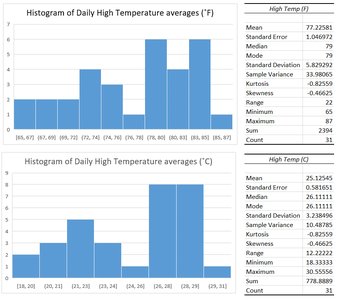
• Application: Standardization allows for comparison across different units of measure, such as Fahrenheit and Celsius for temperature.

The Normal Model

Introduction to the Normal Model

The Normal model (or Normal distribution) is a mathematical model that describes distributions that are unimodal and symmetric. It is used extensively in statistics to model real-world phenomena.

• Notation: A Normal model with mean $\mu$ and standard deviation $\sigma$ is written as $N(\mu, \sigma)$.

• Standard Normal Model: When data is standardized, it follows the Standard Normal Model, denoted as $N(0, 1)$.

The 68-95-99.7 Rule

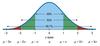
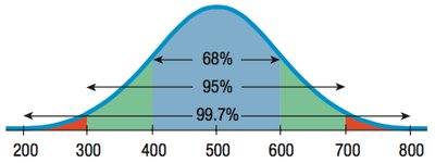
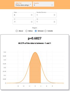
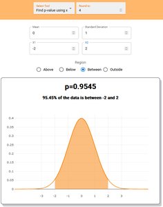
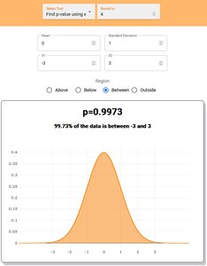
The 68-95-99.7 Rule (Empirical Rule) describes the percentage of data within 1, 2, and 3 standard deviations from the mean in a Normal distribution:

• About 68% of data falls within 1 standard deviation of the mean.

• About 95% falls within 2 standard deviations.

• About 99.7% falls within 3 standard deviations.

Identifying Unusual Values

A z-score with an absolute value greater than 3 is considered "big" or unusual. Such values are often called outliers. For example, z-scores of 10 or more (as seen with world record heights) are extremely rare and represent extreme outliers.

Checking the Normality Assumption

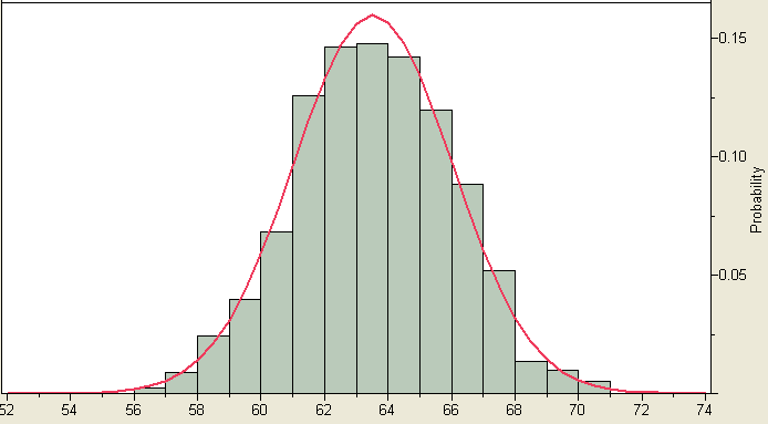
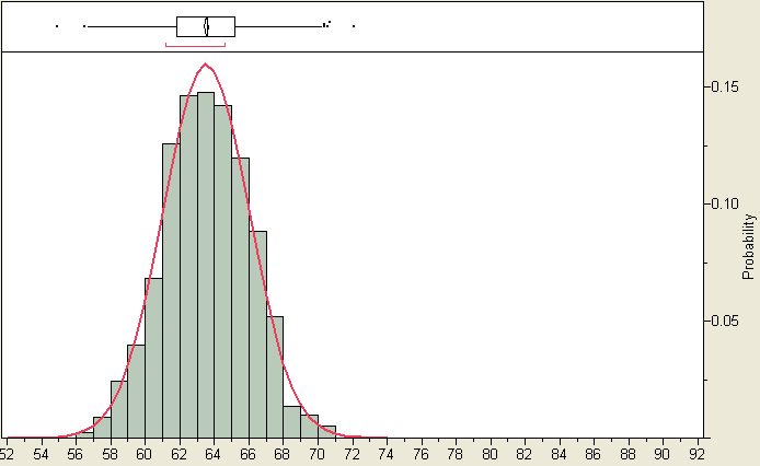
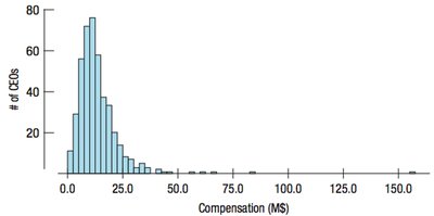
Before applying the Normal model, it is important to check if the data is approximately Normal. The Nearly Normal Condition requires the distribution to be unimodal and symmetric. This can be checked visually using a histogram.

Working with Normal Percentiles

Percentiles and Quantiles

A percentile indicates the value below which a given percentage of observations fall. For example, the 50th percentile is the median. Quartiles (Q1, Q3) are the 25th and 75th percentiles, respectively.

Finding Normal Percentages Using Technology

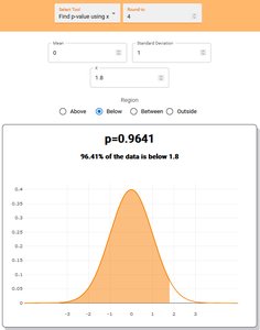
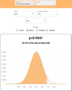
Statistical calculators and software can compute the percentage of data within a given range for a Normal distribution. For example, if SAT scores are normally distributed with mean 500 and standard deviation 100, a score of 680 (z = 1.8) is higher than about 96.4% of the population.

Example: Body Temperature

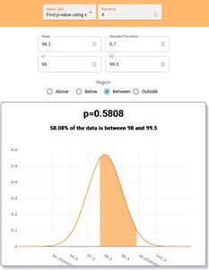
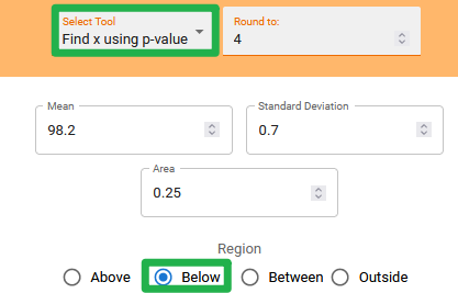
Suppose body temperature is normally distributed with mean 98.2°F and standard deviation 0.7°F. We can use the Normal model to answer questions such as:

• What is the z-score for a temperature of 100.0°F?

• What percent of people have temperatures above 100.0°F?

• What percent have temperatures between 98.0°F and 99.5°F?

Finding Values for Given Percentiles

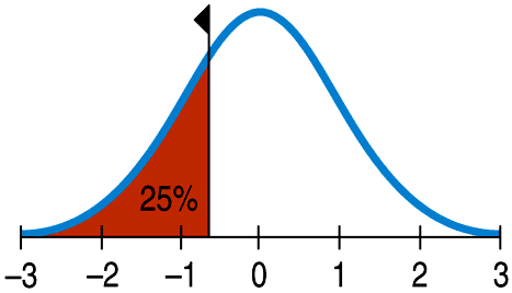
To find the value corresponding to a given percentile (e.g., the first quartile or the coolest 25% of people), use the inverse Normal calculation.

Assessing Normality: Normal Probability Plots

Normal Probability (Quantile) Plots

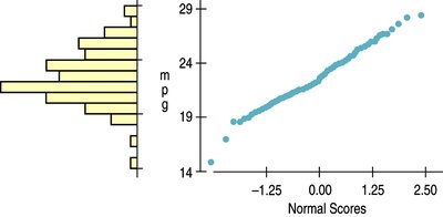
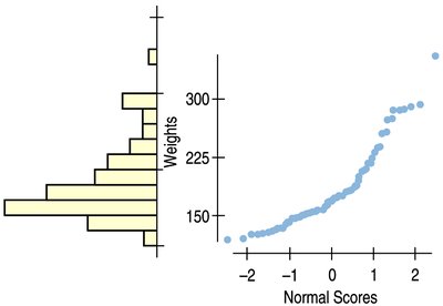
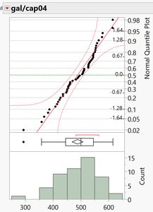
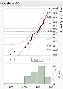
A Normal probability plot (or Normal quantile plot) is a graphical tool to assess whether data is approximately Normal. If the points fall roughly along a straight line, the data is likely Normal. Deviations from the line indicate departures from Normality.

Goodness of Fit Test for Normality

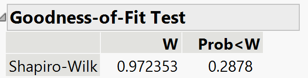
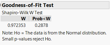
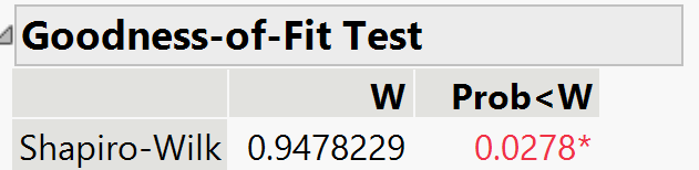
The Goodness of Fit Test (such as the Shapiro-Wilk test) provides an objective criterion for assessing Normality. The test produces a p-value; if the p-value is less than a chosen threshold (commonly 0.05), we reject the assumption of Normality.

Test	W	Prob < W (p-value)
Shapiro-Wilk (2004 data)	0.972353	0.2878
Shapiro-Wilk (2000 data)	0.9478229	0.0278*

Chapter Example: Tire Life

Example Applications of the Normal Model

• Suppose: Tire tread life is normally distributed with mean 32,000 miles and standard deviation 2,500 miles.

• Question 1: What percent of tires last between 30,000 and 35,000 miles?

• Question 2: If the company wants to guarantee only 2% of tires, how many miles should they guarantee?

These questions are solved using z-scores and the Normal model to find probabilities and cutoff values.