Time Series Analysis and Forecasting in Econometrics: Concepts, Methods, and Applications

Time Series Data and Forecasting

Prediction vs. Causation

In time series econometrics, it is crucial to distinguish between prediction (forecasting) and causation. Forecasting focuses on predicting future values based on past observations, while causal analysis seeks to understand the effect of one variable on another. For forecasting, the primary goal is accuracy in out-of-sample predictions, not causal interpretation of coefficients.

Types of Time Series Data Transformations

• Levels: The raw values of a variable over time.

• Differences (First Differences): The change in the variable from one period to the next, denoted as $\Delta Y_t = Y_t - Y_{t-1}$.

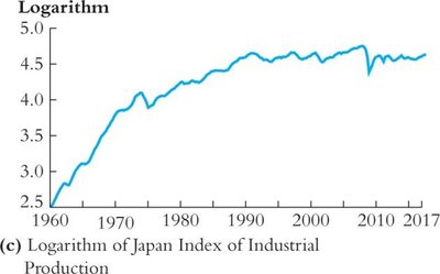
• Logarithms: The natural log transformation, often used to stabilize variance and interpret growth rates.

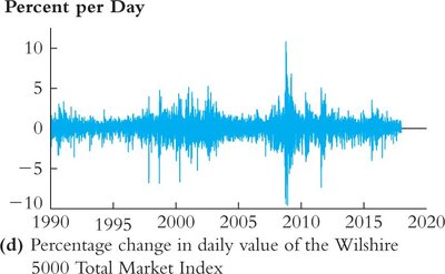
• Percent Changes: The percentage change from one period to the next, often approximated by $100 \times \Delta \ln(Y_t)$ for small changes.

• Changes in Logarithms: $\Delta \ln(Y_t) = \ln(Y_t) - \ln(Y_{t-1})$.

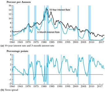
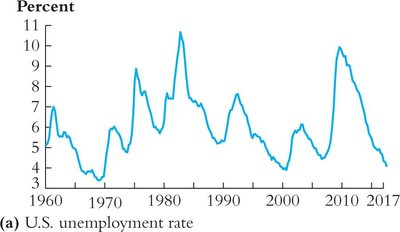
• Portion of the Total: Expressing a variable as a percentage of a total (e.g., unemployment rate).

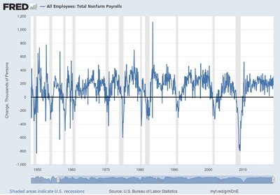
Example: Data in First Differences

The first difference transformation is commonly used to analyze changes rather than levels, especially when the data exhibit trends or nonstationarity.

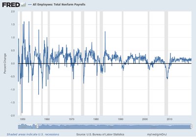
Example: Changes in Logarithms, % Change

Taking the difference of logarithms approximates the percentage change, which is useful for interpreting growth rates in economic data.

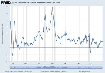
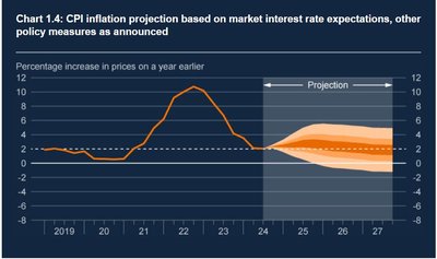
Example: Consumer Price Index (CPI) Changes

Year-over-year percent changes in the CPI are used to measure inflation.

Lagging the Data and Autocorrelation

Lags and Differences

• Lag: The value of a variable from a previous period, e.g., the first lag is $Y_{t-1}$.

• First Difference: $\Delta Y_t = Y_t - Y_{t-1}$.

• First Difference of Logarithm: $\Delta \ln(Y_t) = \ln(Y_t) - \ln(Y_{t-1})$.

• Percentage Change Approximation: $100 \times \Delta \ln(Y_t)$.

Autocorrelation (Serial Correlation)

Autocorrelation measures the correlation of a time series with its own past values. It is a key concept in time series analysis, indicating the persistence of shocks over time.

• First Autocovariance: $\mathrm{Cov}(Y_t, Y_{t-1})$

• First Autocorrelation: $\rho_1 = \mathrm{corr}(Y_t, Y_{t-1}) = \frac{\mathrm{cov}(Y_t, Y_{t-1})}{\sqrt{\mathrm{var}(Y_t)\mathrm{var}(Y_{t-1})}}$

• j-th Autocorrelation: $\rho_j = \mathrm{corr}(Y_t, Y_{t-j})$

Forecasting Models and Stationarity

Forecasting Basics

Forecasting uses historical data to predict future values. The accuracy of forecasts depends on the similarity between the historical (in-sample) and future (out-of-sample) periods, a property known as stationarity.

Stationarity

A time series is stationary if its probability distribution does not change over time. Stationarity is essential for reliable forecasting, as it ensures that the relationships observed in the past persist into the future.

• Strict Stationarity: The joint distribution of $(Y_{s+1}, ..., Y_{s+T})$ does not depend on $s$.

• Joint Stationarity: Two series $X_t$ and $Y_t$ are jointly stationary if their joint distribution does not depend on $s$.

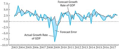
Forecasts and Forecast Errors

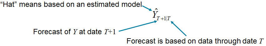
• Forecast: An out-of-sample prediction, e.g., $\hat{Y}_{T+1|T}$ is the forecast for $Y_{T+1}$ based on data through $T$.

• Forecast Error: $e_{T+1} = Y_{T+1} - \hat{Y}_{T+1|T}$

• Mean Squared Forecast Error (MSFE): $MSFE = E[(Y_{T+1} - \hat{Y}_{T+1|T})^2]$

Autoregressive and ADL Models

Autoregressive (AR) Models

An autoregressive model predicts a variable using its own past values. The order of the model, $p$, indicates how many lags are included.

• AR(1) Model: $Y_t = \beta_0 + \beta_1 Y_{t-1} + u_t$

• AR(p) Model: $Y_t = \beta_0 + \beta_1 Y_{t-1} + \cdots + \beta_p Y_{t-p} + u_t$

Autoregressive Distributed Lag (ADL) Models

The ADL model extends the AR model by including lagged values of other predictors (X variables):

• ADL(p, q) Model: $Y_t = \beta_0 + \beta_1 Y_{t-1} + \cdots + \beta_p Y_{t-p} + \delta_1 X_{t-1} + \cdots + \delta_q X_{t-q} + u_t$

Model Selection and Forecast Evaluation

Information Criteria for Lag Selection

Choosing the appropriate lag length is crucial for model performance. Two common criteria are:

• Bayesian Information Criterion (BIC): $BIC(p) = \ln\left(\frac{SSR(p)}{T}\right) + \frac{(p+1)\ln T}{T}$

• Akaike Information Criterion (AIC): $AIC(p) = \ln\left(\frac{SSR(p)}{T}\right) + \frac{2(p+1)}{T}$

BIC penalizes model complexity more heavily than AIC, often resulting in more parsimonious models.

Forecast Intervals and Uncertainty

• Root Mean Squared Forecast Error (RMSFE): $RMSFE = \sqrt{E[(Y_{T+1} - \hat{Y}_{T+1|T})^2]}$

• Forecast Interval (95%): $\hat{Y}_{T+1|T} \pm 1.96 \times \widehat{RMSFE}$

Nonstationarity: Trends and Structural Breaks

Trends in Time Series Data

A trend is a persistent, long-term movement in a time series. Trends can be deterministic (e.g., linear) or stochastic (random walk).

• Deterministic Trend: $Y_t = \alpha + \beta t$

• Stochastic Trend (Random Walk): $Y_t = Y_{t-1} + u_t$

Unit Roots and the Dickey-Fuller Test

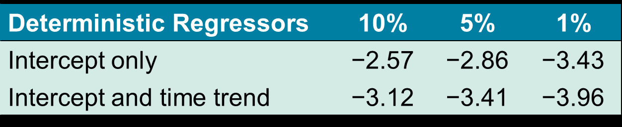
A unit root in an AR(1) model ($\beta_1 = 1$) implies a stochastic trend. The Dickey-Fuller test is used to test for unit roots:

• DF Test Regression: $\Delta Y_t = \beta_0 + \delta Y_{t-1} + u_t$

• Null Hypothesis: $\delta = 0$ (unit root, nonstationary)

• Alternative Hypothesis: $\delta < 0$ (stationary)

Structural Breaks and Model Stability

Testing for Structural Breaks

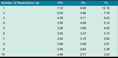
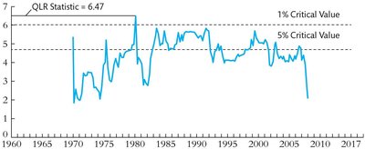
Structural breaks occur when the relationship between variables changes over time. The Chow test (for known break dates) and the Quandt Likelihood Ratio (QLR) test (for unknown break dates) are used to detect such breaks.

• Chow Test: Tests for parameter stability at a known break date.

• QLR Test: Maximum of Chow F-statistics over a range of possible break dates.

Pseudo Out-of-Sample (POOS) Forecasting

POOS forecasting simulates real-time forecasting by re-estimating the model as new data become available and comparing forecasts to actual outcomes. This method is useful for assessing model stability, especially at the end of the sample.

Summary Table: Key Concepts and Formulas

Concept	Formula / Description
First Difference	$\Delta Y_t = Y_t - Y_{t-1}$
Log Difference (Approx. % Change)	$\Delta \ln(Y_t) \approx \frac{Y_t - Y_{t-1}}{Y_{t-1}}$
AR(1) Model	$Y_t = \beta_0 + \beta_1 Y_{t-1} + u_t$
ADL(p, q) Model	$Y_t = \beta_0 + \sum_{i=1}^p \beta_i Y_{t-i} + \sum_{j=1}^q \delta_j X_{t-j} + u_t$
Forecast Error	$e_{T+1} = Y_{T+1} - \hat{Y}_{T+1|T}$
MSFE	$MSFE = E[(Y_{T+1} - \hat{Y}_{T+1|T})^2]$
RMSFE	$RMSFE = \sqrt{MSFE}$
BIC	$BIC(p) = \ln\left(\frac{SSR(p)}{T}\right) + \frac{(p+1)\ln T}{T}$
AIC	$AIC(p) = \ln\left(\frac{SSR(p)}{T}\right) + \frac{2(p+1)}{T}$