Time Series Data Types, Transformations, and Autocorrelation in Statistics

Time Series Data Types and Transformations

Prediction vs. Causation

In statistical analysis, especially in econometrics and time series, it is important to distinguish between prediction and causation. Prediction focuses on forecasting future values based on past data, while causation aims to understand the underlying relationships between variables.

• Prediction: Uses historical data to estimate future values.

• Causation: Investigates whether changes in one variable cause changes in another.

• Forecasting: Can be based on past values, other time series, or a combination.

Types of Time Series Data

Time series data can be represented in various forms, each providing different insights and statistical properties. Understanding these types is crucial for proper analysis and modeling.

• Levels: The raw values of the variable over time.

• Differences: Changes in levels between consecutive periods.

• Logarithms: The natural log transformation of the data, often used to stabilize variance.

• Percent Changes: The percentage change from one period to the next.

• Changes in Logarithms: Approximates percent changes for small values.

• Portion of the Total: Expresses data as a fraction or percentage of a total.

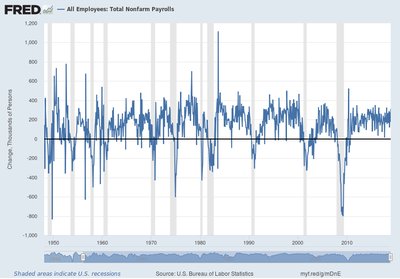
Data in Levels

Data in levels refers to the original, untransformed values of a time series. This form is useful for observing long-term trends and absolute changes.

• Example: Number of employees on nonfarm payrolls over time.

• Application: Used to identify overall growth or decline.

Data in First Differences

The first difference of a time series measures the change between consecutive periods. This transformation is often used to analyze short-term fluctuations and remove trends.

• Formula: $\Delta Y_t = Y_t - Y_{t-1}$

• Application: Useful for stationarity and volatility analysis.

Data in Logarithms

Applying the natural logarithm to time series data can stabilize variance and make multiplicative relationships additive. Log transformation is common in economic and financial data.

• Formula: $\ln(Y_t)$

• Application: Used for growth rate analysis and modeling proportional changes.

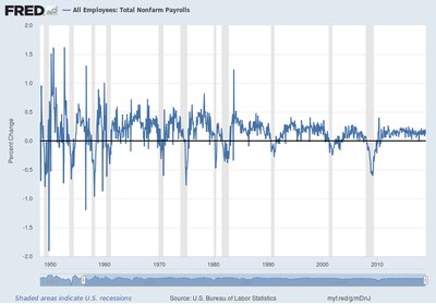
Changes in Logarithms and Percent Change

The change in logarithms between periods approximates the percent change, especially for small values. This is a fundamental concept in time series analysis.

• Formula: $\Delta \ln(Y_t) = \ln(Y_t) - \ln(Y_{t-1})$

• Percent Change Approximation: $100 \times \Delta \ln(Y_t) \approx \frac{Y_t - Y_{t-1}}{Y_{t-1}} \times 100$

• Application: Used for analyzing growth rates and returns.

Portion of the Total

Some time series are expressed as a portion or percentage of a total, which is useful for understanding relative contributions or shares.

• Example: Unemployment rate as a percentage of the labor force.

• Application: Used for ratio analysis and comparisons.

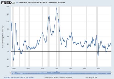
Levels and Changes: Consumer Price Index Example

Time series data for indices, such as the Consumer Price Index (CPI), are often analyzed in terms of both levels and changes. Changes in CPI reflect inflation rates.

• Formula for Percent Change: $\frac{CPI_t - CPI_{t-1}}{CPI_{t-1}} \times 100$

• Application: Used to measure inflation and price stability.

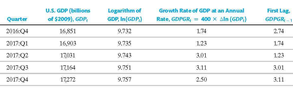
Example: GDP Growth Rate Calculation

Growth rates are commonly calculated using both raw differences and logarithmic approximations. For quarterly GDP, the annualized growth rate is often used.

• Formula: $\text{GDP Growth Rate} = 100 \times \frac{GDP_{t} - GDP_{t-1}}{GDP_{t-1}}$

• Annual Rate: Multiply quarterly rate by 4.

• Logarithmic Approximation: $4 \times 100 \times [\ln(GDP_t) - \ln(GDP_{t-1})]$

• Example: If GDP in 2016:Q4 is 16,851 and in 2017:Q1 is 16,903, the percentage change is $100 \times \frac{16,903 - 16,851}{16,851} = 0.31\%$.

Lagging the Data

Lags are previous values of a time series, used to model temporal dependencies and predict future values. Lagged variables are essential in autoregressive models.

• First Lag: $Y_{t-1}$

• j-th Lag: $Y_{t-j}$

• Application: Used in forecasting and autocorrelation analysis.

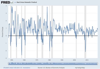
Example: GDP, % Change, Lagged

The quarterly rate of GDP growth is calculated as the first difference of the logarithm, converted to percentage points at an annual rate by multiplying by 400. The first lag is its value in the previous quarter.

• Formula: $GDPGR_t = 400 \times \Delta \ln(GDP_t)$

• Table: Shows GDP, log(GDP), growth rate, and lagged growth rate for several quarters.

Quarter	U.S. GDP (billions of $2009), GDPt	Logarithm of GDP, ln(GDPt)	Growth Rate of GDP at an Annual Rate, GDPGRt = 400 × Δln(GDPt)	First Lag, GDPGRt-1
2016:Q4	16,851	9.732	1.74	2.74
2017:Q1	16,903	9.735	1.23	1.74
2017:Q2	17,031	9.743	3.01	1.23
2017:Q3	17,164	9.751	3.11	3.01
2017:Q4	17,272	9.757	2.50	3.11

Autocorrelation in Time Series

Definition and Importance

Autocorrelation, also known as serial correlation, measures the correlation between a time series and its lagged values. It is a key concept in time series analysis, indicating persistence or patterns over time.

• First Autocovariance: $Cov(Y_t, Y_{t-1})$

• First Autocorrelation: $Cor(Y_t, Y_{t-1})$

• Formula: $corr(Y_t, Y_{t-1}) = \frac{cov(Y_t, Y_{t-1})}{\sqrt{var(Y_t) var(Y_{t-1})}} = \rho_1$

• Population Correlations: Describe the joint distribution of (Y_t, Y_{t-1}).

Autocorrelation at the j-th Lag

The j-th autocovariance and autocorrelation coefficient generalize the concept to any lag j.

• j-th Autocovariance: $cov(Y_t, Y_{t-j})$

• j-th Autocorrelation: $\rho_j = corr(Y_t, Y_{t-j}) = \frac{cov(Y_t, Y_{t-j})}{\sqrt{var(Y_t) var(Y_{t-j})}}$

Sample Autocorrelations

Sample autocorrelations estimate population autocorrelations using observed data. The conventional definition for time series uses the full sample size as the divisor.

• Sample Autocorrelation: $\hat{\rho}_j = \frac{\hat{cov}(Y_t, Y_{t-j})}{\hat{var}(Y_t)}$

• Sample Covariance: $\hat{cov}(Y_t, Y_{t-j}) = \frac{1}{T} \sum_{t=j+1}^{T} (Y_t - \bar{Y}_{j+1,T}) (Y_{t-j} - \bar{Y}_{1,T-j})$

• Sample Mean: $\bar{Y}_{j+1,T}$ is the sample average over $t = j+1, ..., T$.

Example: Quarterly % Change and Autocorrelation

Sample autocorrelation coefficients for quarterly percentage change in real GDP can be calculated and interpreted. For example, $\hat{\rho}_1 = 0.33$, $\hat{\rho}_2 = 0.26$, $\hat{\rho}_3 = 0.10$, and $\hat{\rho}_4 = 0.11$ indicate moderate persistence in GDP growth rates.

Summary Table: Time Series Data Transformations

Transformation	Formula	Purpose
Level	$Y_t$	Raw data, trend analysis
First Difference	$\Delta Y_t = Y_t - Y_{t-1}$	Short-term changes, stationarity
Logarithm	$\ln(Y_t)$	Variance stabilization, growth rates
Change in Logarithm	$\Delta \ln(Y_t) = \ln(Y_t) - \ln(Y_{t-1})$	Approximate percent change
Percent Change	$100 \times \frac{Y_t - Y_{t-1}}{Y_{t-1}}$	Relative change, returns
Lag	$Y_{t-j}$	Temporal dependence, forecasting
Autocorrelation	$\rho_j = corr(Y_t, Y_{t-j})$	Persistence, time series structure

Key Takeaways

• Time series data can be transformed in multiple ways to reveal different statistical properties.

• Logarithmic and difference transformations are essential for analyzing growth rates and stationarity.

• Autocorrelation measures the relationship between current and past values, crucial for forecasting and model selection.

• Sample autocorrelations provide empirical estimates of persistence in time series.