Understanding and Comparing Distributions in Introductory Statistics

Understanding and Comparing Distributions

Introduction to Comparing Distributions

In statistics, comparing distributions is essential for understanding differences and similarities between groups or datasets. This process involves examining the shape, center, and spread of data, often using graphical and numerical summaries.

Displays for Comparing Groups

Histograms for Group Comparison

Histograms are graphical representations that show the distribution of a quantitative variable. When comparing groups, it is crucial to use the same horizontal scale for each histogram to ensure valid comparisons.

• Shape: Describes the overall appearance (e.g., symmetric, skewed, unimodal, bimodal).

• Center: Indicates the typical value (e.g., mean or median).

• Spread: Measures the variability (e.g., range, interquartile range, standard deviation).

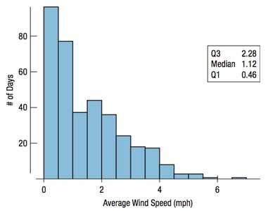
Example: The histogram above shows the distribution of average wind speeds in Hopkins Forest. The distribution is right-skewed, with most days having lower wind speeds.

Comparing Seasonal Distributions

To compare wind speeds between Spring/Summer and Fall/Winter, side-by-side histograms are used. This allows for visual comparison of modality, symmetry, and unusual features.

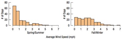
• Modality: Both distributions are unimodal.

• Symmetry: Both are right-skewed, but winter is less skewed than summer.

• Unusual Features: Winter has a broader spread and higher center.

Numerical Summaries for Group Comparison

Numerical summaries such as the mean, median, standard deviation, and interquartile range (IQR) provide quantitative measures for comparing groups.

Season	Mean	StdDev	Median	IQR
Summer	1.11	1.10	0.71	1.27
Winter	1.90	1.29	1.72	1.82

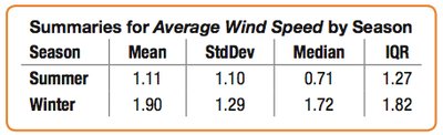
Interpretation: Winter is windier and more variable than summer, as shown by higher mean, median, and IQR values.

Importance of Common Scales in Histograms

When comparing histograms, always use the same horizontal scale. This ensures that differences are not due to scale discrepancies but reflect actual differences in the data.

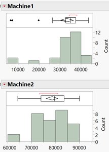
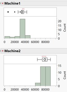
Example: The second set of histograms (with common scales) makes differences between the two machines clearer.

Describing Data Numerically

The 5-Number Summary

The 5-number summary provides a concise overview of a quantitative variable:

• Minimum value

• First quartile (Q1) – 25th percentile

• Median – 50th percentile

• Third quartile (Q3) – 75th percentile

• Maximum value

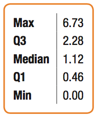
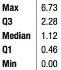
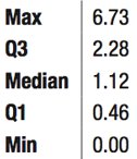
Example: For daily average wind speeds, the 5-number summary is:

• Min: 0.00

• Q1: 0.46

• Median: 1.12

• Q3: 2.28

• Max: 6.73

Boxplots

Introduction to Boxplots

A boxplot is a graphical summary of a quantitative variable, constructed from the 5-number summary. Boxplots provide a balance of information and simplicity, making them ideal for comparing groups.

Constructing Boxplots

1. Draw a vertical axis spanning the data range.

2. Draw horizontal lines at Q1, median, and Q3.

3. Connect these lines to form a box.

4. Erect "fences" at Q1 - 1.5(IQR) and Q3 + 1.5(IQR) to identify potential outliers.

5. Draw "whiskers" from the box to the most extreme data points within the fences.

6. Mark outliers beyond the fences with special symbols.

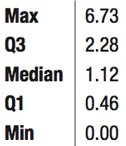
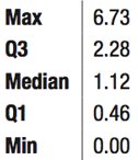
Note: The final boxplot does not display the fences, only the box, whiskers, and outliers.

Comparing Histograms and Boxplots

Histograms and boxplots both display distributions, but in different ways. Histograms show the shape and frequency of data, while boxplots summarize the center, spread, and outliers.

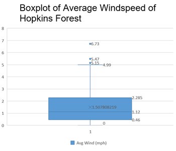
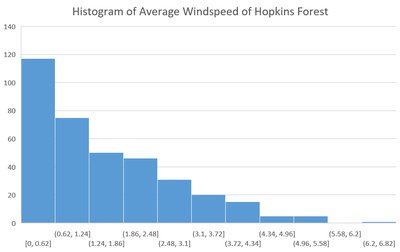
Example: The histogram reveals the skewness and modality, while the boxplot highlights the median, quartiles, and outliers.

Boxplots for Comparing Multiple Groups

Boxplots are especially useful for comparing several groups side by side. They allow for quick visual comparison of medians, spreads, and potential outliers across groups.

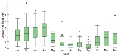
Example: The boxplots above show monthly wind speed distributions, revealing which months are windier and more variable.

Outliers

Identifying and Handling Outliers

Outliers are data points that fall far from the rest of the distribution. They deserve special attention because they may indicate data errors, unusual conditions, or important phenomena.

• Investigate the cause of outliers (e.g., data entry errors, misunderstanding, or genuine extreme values).

• Never ignore outliers; if they are errors, correct them. If removed, document and justify the removal.

• If unsure, analyze data both with and without outliers and report both results.

Outliers and Data Errors

Common causes of outliers due to errors include:

• Transposed digits or data entry mistakes

• Misunderstood survey questions

• Confusion about units of measure

• Cheating or intentional misreporting

Outliers in Practice: Kentucky Derby Example

Winning times in the Kentucky Derby provide a real-world example of outliers. The range of times can be affected by changes in race distance or other factors.

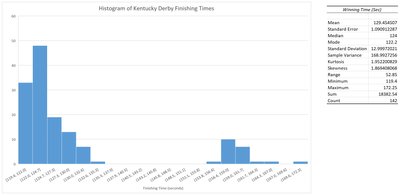
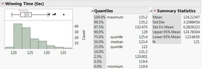
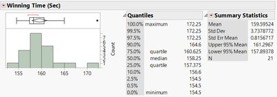
Example: The change in race distance from 1.5 miles to 1.25 miles creates two distinct distributions, each with its own range and potential outliers.

Summary Table: Key Comparisons

Display	Best For	Key Features
Histogram	Comparing 1-2 groups	Shows shape, modality, skewness, and frequency
Boxplot	Comparing 2+ groups	Shows median, quartiles, spread, and outliers

Additional info: Boxplots are preferred for comparing multiple groups due to their compactness and ability to display summary statistics side by side.